Eigenmode tracking theory

A broadband source interpolates between fields solved at different frequencies. Before it can do that, it must establish which fields belong together. Three examples explain why:

• In an anisotropic guide, two propagation curves can cross. The same physical field can move from the first to the second position in the solver’s list. Field matching follows that mode through the crossing.

• For a circular TE11 pair, x/y fields and two diagonal fields are equally valid ways to describe the same degenerate pair. Subspace alignment chooses consistent representatives before interpolating them.

• An artificial outer boundary can support or distort a mode. A successful eigenvalue solve does not establish that the profile represents the intended open guide. Mesh/window comparisons provide separate evidence and warnings; they do not automatically remove a usable profile.

The worked explanations and user controls are in Eigenmode tracking guide. This section gives the mathematics behind them. Select automatic tracking per port with tracking="auto". anchors independently selects the primary solve frequencies.

The automatic pipeline has five stages: solve primary anchors with extra internal candidates; assign branch identities outwards from the reference anchor; resolve ambiguity with midpoint solves; orient eligible degenerate groups; and evaluate numerical, confinement, and artifact diagnostics. The resulting bank supplies injection, receiver decomposition, cached studies, and inspection plots. These stages do not collapse into a single valid/invalid flag: a boundary-sensitive profile may remain usable even though its confinement evidence is poor.

With tracking="auto", public labels are seeded at the solved anchor nearest the band center, choosing the lower frequency on a tie. Tracking proceeds outwards in both directions using complex E/H overlap and a prediction of the next eigenvalue. It uses the physical fields of the 1D and 2D solvers with their Yee sampling and numerical-dispersion conventions. One-to-one assignment includes an explicit unmatched state; an ambiguous assignment is not forced merely to keep a mode number present. Extra internal candidates, including missing degenerate partners, do not create additional public source or monitor channels. extra_candidates requests four additional eigenpairs per solve by default, bounded by the available free degrees of freedom. Hidden partners complete the internal group while modes continues to define the public channels.

Field overlap and eigenvalue prediction

Field overlap measures how similar two patterns are after ignoring an arbitrary overall phase. It allows an x-like mode to match the next x-like mode even when their raw solution numbers differ. The propagation-constant trend provides another clue; neither the list position nor that trend alone decides the match.

For candidate \(i\) at anchor \(k\), concatenate the native physical electric and impedance-scaled magnetic fields into a normalized column:

\[q_{k,i} = \frac{(\mathbf E_{k,i},\eta_0\mathbf H_{k,i})} {\|(\mathbf E_{k,i},\eta_0\mathbf H_{k,i})\|_2}, \qquad O_{ij}=|q_{k,i}^{\mathrm H}q_{k+1,j}|^2.\]

The squared overlap is insensitive to arbitrary complex phase and is clipped to \([0,1]\) against round-off. Invalid or nonfinite field columns cannot provide a valid matched anchor. With two previously tracked anchors, the native eigenvalue is predicted by linear extrapolation in frequency:

\[\widehat\lambda_i(f_{k+1}) = \lambda_i(f_k) + \frac{f_{k+1}-f_k}{f_k-f_{k-1}} [\lambda_i(f_k)-\lambda_i(f_{k-1})].\]

The first step uses the previous eigenvalue without extrapolation. The same rule applies while traversing anchors toward lower frequencies. For an individual-mode candidate, the assignment cost is

\[\begin{split}d_{ij} &= \frac{|\lambda_j(f_{k+1})-\widehat\lambda_i(f_{k+1})|} {\max(1,|\lambda_i(f_k)|)},\\ C_{ij} &= 1-O_{ij}+0.1\min(d_{ij}^2,4).\end{split}\]

Candidates below tracking_overlap (default squared overlap 0.8) are excluded. Additional unmatched columns have cost unmatched_cost (0.65). A minimum-total-cost one-to-one assignment prevents two public labels from claiming the same candidate. For each proposed individual match, the solver repeats assignment with that edge forbidden. The increase in total cost must be at least assignment_margin (0.02); otherwise the identity remains unmatched. Thus a locally strong overlap is insufficient if an almost equally good competing assignment exists.

SVD rank checks and principal-angle comparison

For TE11, comparing only the first returned field can mistake a harmless rotation from x/y to diagonal polarizations for a change of mode. Instead we compare all fields that the pair can form together: their subspace. SVD provides a well-conditioned basis for that comparison, independent of the particular pair the eigensolver returned.

A degenerate eigenvalue defines a space of valid fields, rather than a unique set of individual eigenvectors. An eigensolver may return any invertible combination of a basis for that space, including nonorthogonal columns. Normalizing each column alone therefore cannot make a subspace comparison independent of the solver’s basis.

Let \(F\in\mathbb C^{N\times r}\) contain the flattened E/H field columns for an \(r\)-mode group. Candidate assignment uses the normalized columns \(q_i\) above; alignment uses the full E/H frame at its current scaling. The reduced singular value decomposition (SVD) is

\[F=U\Sigma V^{\mathrm H},\qquad \Sigma=\operatorname{diag}(s_1,\ldots,s_r),\qquad s_1\ge\cdots\ge s_r\ge0.\]

The implementation requires finite singular values and \(s_r>s_1/10^8\). It rejects rank loss or excessive conditioning instead of silently dropping a partner and changing the group’s dimension. The orthonormal span basis and its transformation from the input columns are

\[Q=U,\qquad B=V\Sigma^{-1},\qquad FB=Q,\qquad Q^{\mathrm H}Q=I.\]

This Euclidean E/H normalization compares spans and conditions the power check; it does not by itself give unit transported power.

For equal-rank spans at two anchors, a second SVD gives their principal angles:

\[Q_a^{\mathrm H}Q_b=L\,\operatorname{diag}(\sigma_1,\ldots,\sigma_r) R^{\mathrm H},\qquad \sigma_i=\cos\theta_i.\]

The smallest singular value measures the least well matched direction. The automatic candidate-assignment score is

\[O_{\mathrm{span}} = \sigma_{\min}^2(Q_a^{\mathrm H}Q_b).\]

Identical spans have score one even if their input columns have unrelated phases, ordering, rotations, or nonorthogonal bases. A missing or substantially changed direction lowers the smallest singular value even when the other directions match well. Assignment compares the squared score against tracking_overlap (default 0.8). The later aligned-group continuity check uses the unsquared \(\sigma_{\min}\) with its separate 0.9 warning and 0.6 rejection thresholds.

Candidate clusters and adaptive frequency solves

The candidate gap cluster_gap (1e-5) is an upper limit on grouping, not evidence that every nearby mode belongs to one degenerate eigenspace. Span reservation uses whole-group eigenvalue spreads no larger than the smaller of this gap and the 1e-8 degeneracy tolerance. Previously tracked members must meet that bound in both their last solved and predicted eigenvalues; new groups are checked at the new anchor. Complete-link admission prevents a chain of close eigenvalues from joining resolved endpoints.

A persistent pair may temporarily share an eigenvalue cluster with a crossing branch. When group sizes differ, project each column of the larger group onto the smaller span, and select as many columns as the smaller span’s dimension. The squared projection scores of the last selected and first excluded columns must differ by at least subspace_margin (0.02). The selected equal-size spans must then pass the usual smallest-principal-angle overlap test. The operation is symmetric for merging and splitting clusters. Group selection remains sequential, prioritizing the largest admissible match, then assignment cost and overlap; there is no global group-assignment margin. Matched members are reserved, and remaining modes enter individual assignment. No fields are mixed by this subset-selection step.

At a crossing, the eigensolver can return arbitrary combinations of all coincident modes. A recovery pass first continues the fields from a resolved neighbor through this full span. If \(Q\) is an orthonormal basis for the new cluster, \(F\) contains its original E/H columns, and \(R\) contains the neighboring reference fields, recovery uses

\[Y=QQ^{\mathrm H}R,\qquad T=F^{+}Y.\]

When the cluster merges previously resolved groups, successful raw-column assignment alone does not bypass recovery. Each assigned subgroup must match the projected reference span to a projector tolerance of 1e-8; otherwise the full-span projection above restores its identity. For frequency-dependent subspaces this is a finite-anchor transport approximation; its projector error must be controlled by anchor refinement, even when the mixed eigen-residual vanishes at an exact coincidence.

The same transformation \(T\) is applied to every E/H component. Projection preserves reference subgroups without forcing distinct subgroups to be mutually orthogonal. Recovery requires full rank, sufficient complete-span overlap, compatible propagation roots, and a mixed eigen-residual within residual_tolerance (default 1e-7). Both the reference candidates and the new cluster must pass the solver’s spatial-resolution check when that diagnostic is available; a small eigenproblem residual alone does not establish spatial resolution. The 2D solver also reevaluates the reconstructed transverse and longitudinal Maxwell equations. The accepted fields then enter the usual association procedure. Failed checks follow the normal refinement/failure policy.

Transport starts at the anchor with the least total degeneracy; ties favor the requested reference frequency and then the lower anchor index. Public labels still originate at the requested reference anchor. A recovered cluster can be continued across several consecutive coincident anchors. The HDF5 mode_tracking/subspace_recovery records the original candidate slots, reference slots, transformations, and residuals before final reordering.

Recovery uses field history, without TE/TM labels or spatial symmetry tests. A persistent four-dimensional degeneracy with no resolved neighboring subgroups remains one tracking group. There is no imposed two-mode limit. Automatic detection of the native C4v or C2v symmetry can subsequently decompose its source span into irreducible blocks. Detection uses sampled materials and boundary masks at every anchor, followed by modal closure, power, continuity, and residual checks. If no decomposition passes, the power-whitened source span is retained.

After association, automatic mixing groups are partitioned using their eigenvalue trajectories throughout the solved bank, with the tighter 1e-8 whole-group spread bound at every anchor. This retains persistent subgroups even if the reference anchor coincides with a crossing. Field mixing still requires the propagation-branch, positive-power, rank, and mixed-residual checks in Degenerate subspaces and physical alignment. Independently established groups may share an eigenvalue at a crossing: their complete coincident field bank must remain full rank and have a positive, well-conditioned power form. Each group is whitened separately; the complete bank retains cross-group power terms for receiving decomposition.

The controlled algebraic checks in python -m testing.eigenmode_support.subspaces.persistent_mode_groups --output results.json cover a pair crossed by one mode, two crossing pairs, a resolved crossing inside the broad candidate gap, a four-dimensional degeneracy, and safe recovery at a fully mixed exact crossing. These are association tests, not Maxwell or scattering-accuracy evidence.

The regression suite also checks subgroup projectors at inter-group rotations of 10, 15, and 20 degrees, where assignment can succeed despite mixed fields. For evolving subspaces, halving the anchor spacing halves the historical projection error in the controlled crossing cases.

For broader checks and tracked-branch plots, run python -m testing.eigenmode_support.subspaces.expanded_mode_tracking --output results/tracking. This adds multiple simultaneous and repeated crossings, higher-dimensional groups, resolved splitting, complex eigenvalues with nonorthogonal fields, and avoided crossings under randomized bases and different reference anchors. It also solves full-vector Yee-grid FDFD square-guide material sweeps, with and without dielectric loss, in which a degenerate TE pair crosses a TM mode, a square-guide crossing between the TE20/TE02 and TM12/TM21 degenerate pairs, and an anisotropic rectangular-guide frequency sweep. Independent discrete dispersion formulas check the square-guide modes and the rectangular-guide fundamentals. The material sweeps are independent constitutive models at 20 GHz, not time-domain simulations of a causal dispersive material. Exact coincidences include deliberately rotated eigensolver bases to exercise whole-cluster recovery.

python -m testing.eigenmode_support.subspaces.general_subspace_tracking --output results/subspaces adds a square metallic-guide pair crossing, an inhomogeneous anisotropic dielectric-loaded square PEC guide with crossing hybrid doublets, a square dielectric core in air inside a finite port window, and a persistent metallic fourfold control. It checks final E/H Maxwell residuals, group continuity, per-group power whitening, and the full power matrix, and plots tracked spans and individual fields. These checks validate FDFD tracking and source-basis construction; they do not run a time-domain scattering experiment.

Ambiguous intervals trigger additional candidates and midpoint solves. The default limits are eight refinement levels, a minimum relative frequency step of 1e-5, and 200 additional solves per port, shared with verification. Required primary anchors are not removed to meet that budget. Persistent ambiguity follows the anchor policy: automatic anchors may fall back to a single band-center profile; multiple explicit anchors raise an error. For an ambiguous interval \([f_a,f_b]\), the next frequency is \(f_m=(f_a+f_b)/2\); subdivision stops when \((f_b-f_a)/\max(|f_m|,1\,\mathrm{Hz})\le10^{-5}\) or a configured limit is reached. A midpoint solve uses the same extra-candidate allowance and the assignment is reevaluated across the bank. The current algorithm does not increase that allowance automatically on each retry. Increase extra_candidates explicitly if inspection indicates missing candidates.

For independently tracked modes, the assigned fields are phase-aligned before interpolation using their complex E/H overlap. Degenerate groups instead use the physical-direction or unitary transport rules below. Neither procedure authorizes interpolation through an unresolved assignment. After fallback, the retained center profile is a fixed-profile approximation away from that frequency, and the unresolved interval remains recorded.

Residuals and verification evidence

Numerical validity uses eigenpair and reconstructed Maxwell-equation residuals from the actual discrete operators, with default tolerance 1e-7. For the reduced eigenproblem \(Av=\lambda v\), the eigenpair residual is

\[r_{\mathrm{eig}} = \frac{\|Av-\lambda v\|_2}{\|Av\|_2+\|\lambda v\|_2}.\]

The denominator is protected against zero. The reconstructed-field residual checks the discrete Maxwell equations with the solver’s numerical-dispersion operators; the larger of the eigenpair and field residuals controls numerical validity. A small eigenpair residual alone does not establish a correct reconstructed E/H profile.

Full verification compares propagation constants and E/H fields against a refined transverse mesh and, for open cross-sections, windows padded by approximately 25% and 50% of the original extent. The larger windows use available model geometry at unchanged spacing and exclude PML. Degenerate groups are compared as subspaces. Default acceptance thresholds are normalized beta drift 1e-3, verification overlap 0.999, and outer-edge field-norm fraction 1e-3; physical enclosing walls are distinguished from artificial edges. These controls belong to EigenmodeTrackingConfig.

The propagation-constant comparison uses

\[\delta_\beta = \frac{|\beta_{\mathrm{test}}-\beta_{\mathrm{base}}|} {\max(|\beta_{\mathrm{base}}|,k_0)}.\]

For a degenerate group it uses the mean beta and compares complete spans. Verification fields are compared on the original window after cropping a larger solve or averaging refined cell fields back to the original cells. The edge fraction is the sum of \(|\mathbf E|^2+\eta_0^2|\mathbf H|^2\) in the outer 10% strips (at least one cell per edge), divided by that sum over the full cross-section. This is a field-norm diagnostic, not a leakage-power measurement. A recognized physical PEC/PMC enclosure is not penalized for field near its wall. verification="fast" evaluates residual and edge evidence without the refinement/window comparisons.

Confinement, artifact suspicion, tracking confidence, and propagation/power eligibility are separate diagnostics. Domain sensitivity or appreciable field at an artificial edge can indicate leakage or a truncation/box artifact; mesh sensitivity alone does not establish a spurious mode. Complex beta alone is also not an artifact test. Suspect or incomplete confinement evidence produces a warning that the usable profile remains in use and accuracy may be reduced. Such warnings do not trim anchors, renumber modes, or force tracking fallback.

The resolved bank is shared by injection, monitors, cached studies, and plots. The versioned HDF5 mode_tracking group records candidate mappings, requested/adaptive frequencies, residuals, diagnostic summaries, and unresolved intervals without changing the existing validity-mask meanings. Degenerate transforms are stored in degenerate_groups. The modal-field plots include tracked dispersion and diagnostic status, including in geometry-only runs.

Degenerate subspaces and physical alignment

Polarization means the direction of the integrated transverse electric field, not the direction of every local field vector:

\[\mathbf m_j(f)=\int_{\mathrm{port}}\mathbf E_{t,j}(f)\,dA.\]

At every anchor, the two moment columns form \(M\). Requested real unit directions in the transverse plane form \(D\). The initial transformation is obtained by solving a small linear system:

\[MT_0=D,\qquad \mathbf E'_j=\sum_i\mathbf E_i(T_0)_{ij},\qquad \mathbf H'_j=\sum_i\mathbf H_i(T_0)_{ij}.\]

Applying the same transformation to every E/H component preserves their relative phase. For real forward powers \(p_j>0\), the final transform is

\[T=T_0\operatorname{diag}(p_j^{-1/2}),\qquad MT=D\operatorname{diag}(p_j^{-1/2}).\]

Thus each column has unit real power and a positive real electric moment parallel to its requested direction; its integrated moment need not have unit magnitude. This fixes orientation and phase consistently across ports before interpolation.

The inferred electric-moment directions are orthogonal. The full Hermitian power matrix is retained: for simultaneous coefficients \(c\), total power is \(c^\dagger P c\), which can include interference terms. Continue using multiple EigenmodeExcitation objects with amplitude and phase_deg for coherent combinations; a 90-degree relative phase drives quadrature.

Explicit directions and the automatic electric-moment fallback use this alignment machinery. Native symmetry decomposition uses the power-preserving orientation described in Discrete symmetry and irreducible subspaces. With physical directions, alignment is enforced independently at every anchor; subsequent tracking diagnostics do not rotate those directions. Without usable physical directions, a deterministic reference basis is transported outwards using the SVD rotation below. Legacy modes without a declared group retain independent-mode phase tracking.

Automatic tracking ignores degenerate and detects groups from the solved spectrum. It separates longitudinal families, resolves symmetry subspaces and eligible directional variation, then orients native doublets by electric moments or mirror parity. Explicit mode_polarizations is applied afterward within each resolved doublet, preserving its span. A two-mode parent with no certified subdivision can use independent electric moments; larger unresolved parents cannot be polarized. Legacy tracking applies the direction to its declared pairs without automatic symmetry selection.

Automatic tracking accepts one axis or real transverse vector, or a deprecated explicit direction pair. With one direction, its partner is the positive port-normal axis crossed with it, independently of propagation sign. Both trackers preserve explicit direction pairs, including their signs and valid nonorthogonal directions, with a deprecation warning. Legacy tracking also accepts mode/group mappings. These forms will be removed in gprMax 5.0. See Eigenmode tracking guide for migration examples. Requested diagonal directions need not diagonalize the mirror actions; native parity is certified before this final rotation. Maxwell residuals and complete-bank measurement conditioning are checked again afterward. The default None retains the automatic orientation.

The native discrete eigenvalue spread must be below \(10^{-8}\max(1,\max|\lambda|)\), and mixed-mode relative eigen-residuals must satisfy residual_tolerance (default \(10^{-7}\)). Resolved splitting in a declared group is an error; automatic tracking keeps split branches as independent modes. Propagation constants are preserved individually. Moment condition numbers above \(10^8\) are rejected. A usable electric moment must also exceed \(10^{-12}\) times the absolute transverse-field sample sum multiplied by transverse cell area; this prevents cancellation noise from defining a polarization even when its relative condition number looks benign. Higher-order groups with vanishing integrated E can use generic tracking, but cannot use axis/vector references. Modes on opposite propagation branches are not mixed even if their squared eigenvalues coincide.

Continuity is measured using the smallest principal subspace-overlap singular value: below 0.9 warns, and below 0.6 rejects an in-band match. Legitimate automatic guard trimming and cutoff exclusion apply to the whole group; failed groups never silently fall back member by member. Non-propagating group anchors are excluded from excitation and physical references.

Power conditioning and normalization

For group coefficients \(c\), define the discrete cross-power matrix using the port’s propagation direction \(\hat{\mathbf w}\) and its Yee field quadrature:

\[C_{ij}=\frac12\int (\mathbf E_j\times\mathbf H_i^*)\cdot\hat{\mathbf w}\,dA,\qquad P=\frac{C+C^{\mathrm H}}{2},\qquad P(c)=c^{\mathrm H}Pc.\]

The 1D cross-section uses its corresponding line quadrature and power per unit invariant length. A change of basis \(F\mapsto FT\) transforms this Hermitian power form as \(P\mapsto T^{\mathrm H}PT\).

Testing power directly in a poorly conditioned solver basis can exaggerate conditioning because the quadratic form contains that basis twice. The code first uses the SVD preconditioner \(B=V\Sigma^{-1}\) and tests \(P_B=B^{\mathrm H}PB\). Its eigenvalues must be finite and satisfy \(p_{\min}>p_{\max}/10^8\), ensuring an independent positive-power basis. A small eigenvalue residual does not substitute for this power test.

For generic subspace alignment, the canonical basis described below has transform \(T_c\) and power matrix \(P_c=T_c^{\mathrm H}PT_c=Z\operatorname{diag}(p_j)Z^{\mathrm H}\). The implementation normalizes the complete power form:

\[T=T_cZ\operatorname{diag}(p_j^{-1/2})Z^{\mathrm H},\qquad T^{\mathrm H}PT=I.\]

Physical-direction alignment instead normalizes each column as above. Orthogonal integrated moments do not by themselves guarantee power orthogonality in a general guide; any off-diagonal power terms are retained.

Deterministic basis without electric directions

When integrated electric moments cannot supply a physical orientation, the code constructs a repeatable basis from the subspace projector \(\Pi=QQ^{\mathrm H}\). Let \(e_\ell\) be a coordinate vector in the flattened E/H sample order, and let \(W\) contain the canonical columns already selected. For each unused coordinate, form

\[z_\ell=(I-WW^{\mathrm H})\Pi e_\ell.\]

Choose the largest \(\|z_\ell\|_2\), breaking an exact tie by the lowest coordinate index. Normalize it and multiply by a complex phase so its selected coordinate is positive real. Repeat until there are \(r\) columns. The implementation applies the projector through \(Q\) without forming the dense \(N\times N\) matrix. A missing independent direction is an error.

For the resulting frame \(F_c\), a least-squares solve determines \(T_c=F^\dagger F_c\), so \(FT_c=F_c\) up to numerical precision. Because the projector depends on the span, this construction avoids choosing an orientation from arbitrary raw eigenvectors. The fixed sample ordering defines its convention; it is not a requested physical polarization. Power normalization is then applied before transport.

Unitary SVD transport between anchors

For a fallback group without physical-direction or native parity constraints, let \(A_k=F_kT_k\) be its current power-normalized frame and \(A_p\) the already aligned frame at the preceding anchor along the tracking path. Solve the complex orthogonal Procrustes problem

\[R_*=\underset{R^{\mathrm H}R=I}{\operatorname{argmin}} \|A_kR-A_p\|_{\mathrm F}.\]

Expanding the squared Frobenius norm shows that this is equivalent to maximizing \(\operatorname{Re}\operatorname{tr}(R^{\mathrm H}A_k^{\mathrm H}A_p)\). For the SVD

\[A_k^{\mathrm H}A_p=U_s\Sigma_sV_s^{\mathrm H}, \qquad R_*=U_sV_s^{\mathrm H},\]

update \(T_k\leftarrow T_kR_*\) and \(A_k\leftarrow A_kR_*\). The rotation is applied to all electric and magnetic field components. It preserves unit power because \(R_*^{\mathrm H}IR_*=I\), and it stays inside the same degenerate subspace. Transport starts at the retained anchor nearest the band center (lower frequency on a tie) and proceeds separately toward increasing and decreasing frequencies.

This transport uses the power-normalized frames themselves; the principal angle test above uses Euclidean-orthonormalized spans. The two SVDs answer different questions: whether the spans match, and which allowed orientation best continues the preceding frame. A physically specified or automatically selected electric direction is not subsequently rotated by Procrustes transport. Native symmetry doublets instead retain their mirror parities and continue each channel by a scalar phase.

After the final rotation, the code recomputes the mixed eigenpair residual for each column against its own stored eigenvalue:

\[r_j=\frac{\|A_{\mathrm{op}}(XT)_j-\lambda_j(XT)_j\|_2} {\|A_{\mathrm{op}}(XT)_j\|_2+\|\lambda_j(XT)_j\|_2} \le r_{\mathrm{tol}},\qquad r_{\mathrm{tol}}=10^{-7}\text{ by default}.\]

Here \(X\) contains the raw reduced eigenvectors and \(A_{\mathrm{op}}\) is the actual discrete eigenproblem operator. The common residual_tolerance setting controls input eigenpair, mixed-vector, and available reconstructed-field residual checks. This changes the acceptance policy from released 4.0.1: the general default was 1e-8, and mixed-mode eigen-residual acceptance used a separate fixed 1e-9 limit. The new default is 1e-7, including legacy degenerate groups, so the mixed-mode limit is relaxed by a factor of 100 at the default. Additional reconstructed Maxwell-residual checks impose a separate physical consistency requirement where the solver supplies them. Set EigenmodeTrackingConfig(residual_tolerance=1e-9) to retain the previous mixed-mode limit; this setting also tightens the other residual checks. Propagation constants and eigenvalues are never replaced by a group average to make mixing pass. Mixing resolved splitting or opposite propagation branches remains forbidden; a numerical rotation cannot repair that physical incompatibility.

The aligned bank is shared by single-anchor and broadband sources, monitors, modal studies, virtual guides and plots. HDF5 port groups include degenerate_groups with requested directions, achieved electric moments, transformations, power matrices, eigenvalue spread, condition numbers, residuals, subspace overlaps and retained-anchor flags. Geometry-only modal field exports include the same diagnostics; plot titles show assigned directions.

Discrete symmetry and irreducible subspaces

Symmetry supplies transformations that leave a port eigenproblem unchanged. Within a degenerate span these transformations become small matrices. Reducing those matrices separates the span into invariant blocks: an irreducible subspace has no smaller nonzero subspace preserved by every group operation. An arbitrary-dimensional degenerate group can therefore contain several singlets and doublets, including repeated copies of the same representation.

Why the square transverse Yee grid supports at most C4v

Consider a uniform square transverse lattice with spacing \(h\), with the propagation axis held fixed. A native rotation must map grid samples back to grid samples. In particular, its action on a shortest translation is

\[R_\theta(h,0)=h(\cos\theta,\sin\theta)\in h\mathbb Z^2.\]

The integer components must still have squared length one. They can only be \((\pm1,0)\) or \((0,\pm1)\), giving rotations by multiples of \(90^\circ\). Together with the two axis mirrors and two diagonal mirrors, these operations form C4v. C4v has eight operations: four rotations and four reflections. It is different from C8v, whose fundamental rotation is \(45^\circ\) and which has sixteen operations.

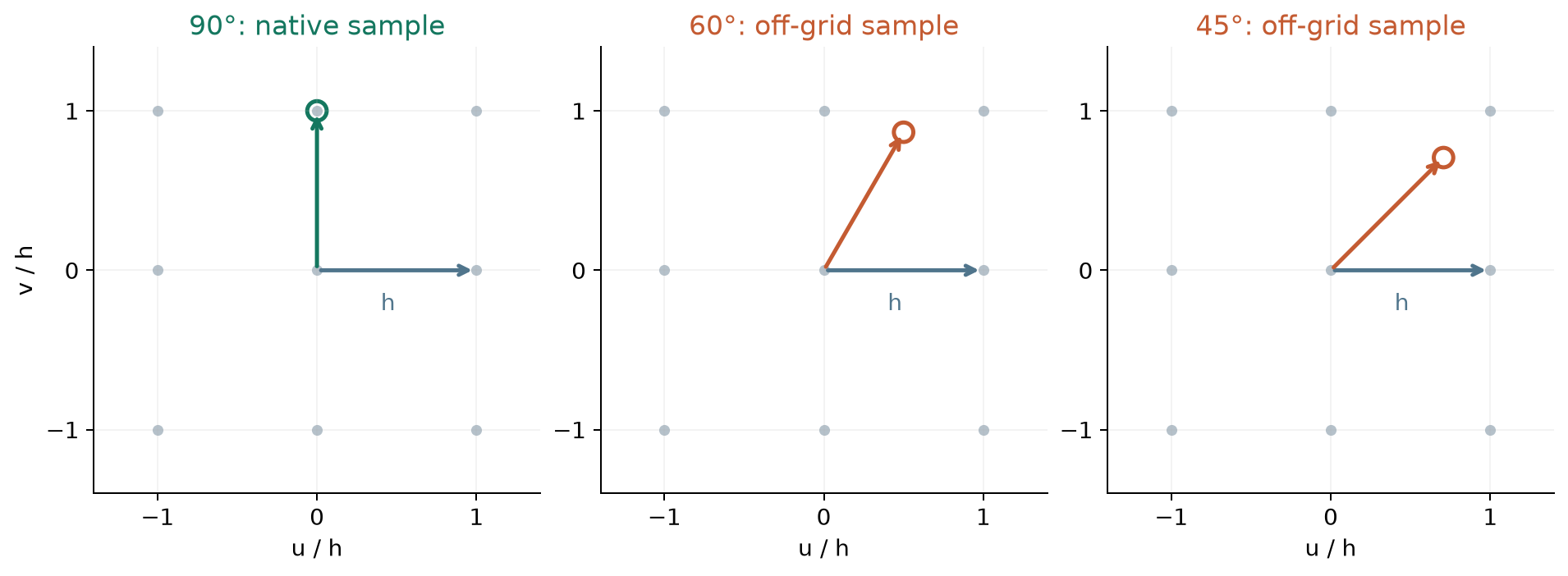
Fig. 20 A quarter turn maps the square lattice onto itself. Rotations by 60 or 45 degrees require interpolation. The illustrated vertices are one Yee sublattice; the field-component transformation also maps the staggered sublattices and applies the vector signs.

A quarter turn exchanges the transverse E components and their staggered locations, and likewise the H components. To preserve the complete discrete problem it must also preserve the material tensors, wall masks, spacing, and aperture. Unequal transverse spacings usually reduce the available group to C2v or a subgroup. Detection tests these sampled quantities at every solved anchor and takes the strongest supported group common to the bank.

This bound concerns rotations and mirrors of a square two-dimensional port cross section, with its normal fixed. A three-dimensional cubic lattice has additional operations that exchange the normal with other axes. Other lattice types have different planar symmetries: a hexagonal lattice admits 60-degree rotations, whereas a square lattice does not [tracking-IUCr].

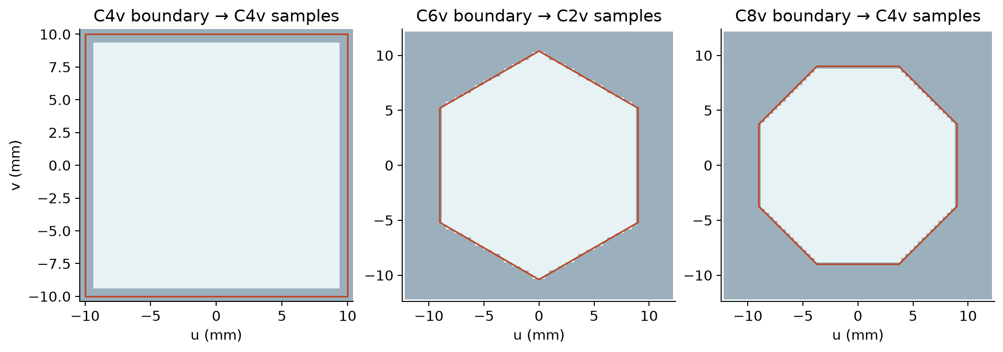
Fig. 21 Ideal boundaries and material samples on square grids. The aligned square retains C4v, the hexagon retains C2v, and the octagon retains C4v. This illustration shows the longitudinal-electric sample mask; detection checks all relevant staggered material and wall arrays.

An ideal circular cross section has continuous rotational symmetry. A centered staircase on a square grid can retain C4v, so some continuum doublets survive and others split. Similarly, the two-dimensional representations of C6v restrict to one-dimensional representations of C2v. For an octagon, the C8v \(E_1\) and \(E_3\) doublets restrict to the C4v \(E\) doublet, whereas \(E_2\) splits into \(B_1\) and \(B_2\). The selected C6v/C8v numerical examples in Simulation examples exhibit both retained degeneracy and splitting. Their resolved branches remain separate under the nominal mixing tolerance.

Vector actions and symmetry validation

For an orthogonal spatial transformation \(R\) acting about the port center, the complete fields transform as

\[(\mathcal S_R\mathbf E)(\mathbf x) =R\mathbf E(R^{-1}\mathbf x),\qquad (\mathcal S_R\mathbf H)(\mathbf x) =\det(R)R\mathbf H(R^{-1}\mathbf x).\]

The determinant accounts for H being an axial vector. For the u-mirror, \(u\mapsto-u\), E has component signs \((-,+,+)\) and H has \((+,-,-)\). Thus the parity of a complete vector mode need not equal the scalar parity of its longitudinal H plot.

For SIBC ports, each installed Ampere row must map to another installed row under these signed field actions. The check compares retained E/H samples, complex relative permittivity, and every magnetic circulation coefficient divided by retained dual area (relative tolerance \(10^{-10}\), absolute \(10^{-12}\)). This includes the frequency-dependent ADE response and clipped corner rows, so equal material names alone do not certify symmetry.

Let \(F\) contain the flattened E/H columns of an eligible group after power whitening. Compute each modal representation by least squares,

\[D_R=F^\dagger\mathcal S_RF,\qquad \mathcal S_RF\simeq FD_R.\]

Check span closure, unitarity, and the group relations with tolerance \(10^{-8}\). For C4v these include \(D_{90}^4=I\), \(D_u^2=I\), and \(D_uD_{90}D_u=D_{90}^{-1}\). Material symmetry alone is insufficient if the supplied modal span omits a required partner; closure detects that case.

The implementation finds the commutant: all matrices \(X\) satisfying

\[XD_R-D_RX=0\quad\text{for every supplied generator }R.\]

These are linear equations solved with SVD. A complex irreducible block has a one-dimensional commutant (scalar multiples of the identity). Otherwise, the eigenspaces of a nonscalar Hermitian commutant element give smaller invariant blocks, and the process repeats. This handles groups of any size. Neighboring subspaces provide a continuation probe for repeated copies; principal-angle matching keeps the selected blocks continuous across anchors.

C4v has four one-dimensional irreducible representations and one two-dimensional representation [tracking-C4v]. C2v has four singlets:

Table 21 Native irreducible subspaces

Symmetry	Blocks	Consequence for a larger degenerate span
C4v	A1, A2, B1, B2 (dimension 1); E (dimension 2)	Can contain several E doublets, singlets, or both. For example, six dimensions may decompose as three doublets.
C2v	A1, A2, B1, B2 (dimension 1)	Simultaneous axis-mirror parity separates singlets.

Repeated equivalent representations admit multiple choices of their copies. The native path first resolves longitudinal-field families as described below, then applies the commutant decomposition within each resolved family. Mirror parity selects partners within each doublet. Compatible equal-parity singlets can subsequently be combined into an axis-oriented source basis. The original irreducible basis and the final source transform are both saved.

Longitudinal-field families

Let \(E_w\) and \(Z_{\rm ref}H_w\) contain native longitudinal field samples, with one column per mode in the power-whitened parent basis. Form

\[L_E=E_w^{\mathrm H}E_w,\qquad L_H=Z_{\rm ref}^2H_w^{\mathrm H}H_w,\qquad M=L_E+L_H, \qquad L_Ec=\rho Mc.\]

The common cell-area factor cancels. Values near zero identify a subspace with negligible longitudinal electric field; values near one identify a subspace with negligible longitudinal magnetic field. In a uniform metallic guide these recover TE and TM families. Intermediate values describe hybrid longitudinal content. The HE/EH naming convention is explained in TE/TM and HE/EH conventions.

The metric must have condition number below \(10^8\) and maximum eigenvalue above \(10^{-12}\|F\|_F^2\), where F is the full E/H frame. Adjacent rho values separated by more than \(10^{-8}\) define distinct families. Each selected family must be invariant under the certified symmetries, within \(10^{-8}\). Singular, insignificant, or unresolved longitudinal fields retain the existing symmetry decomposition.

Each family is power-whitened separately. Cross-family terms remain in the full Hermitian power matrix; whitening the complete bank again would mix the selected physical families. The usual mixed-vector and reconstructed Maxwell residual checks apply to the final E/H fields.

Axis-sensitive selection of equal-parity partners

Some degenerate singlets have the same two mirror parities. For example, the square-guide combinations \(\mathrm{TE}_{20}\pm\mathrm{TE}_{02}\) belong to different rotation irreps but have identical axis-mirror parities. An axis-oriented source basis can recover the individual fields by measuring directional variation. This operation uses the fields, with no prescribed mode indices or analytical templates.

For \(F_E=E_w\) and \(F_H=Z_{\rm ref}H_w\), use native forward differences \(D_u,D_v\), divided by their respective grid spacings:

\[K_u=\sum_{\alpha\in\{E,H\}}(D_uF_\alpha)^{\mathrm H}D_uF_\alpha, \qquad K_v=\sum_{\alpha\in\{E,H\}}(D_vF_\alpha)^{\mathrm H}D_vF_\alpha.\]

Restrict these matrices and M to singlets with matching mirror parities and longitudinal scores agreeing within \(10^{-8}\). The restricted electric matrix must also satisfy \(\|L_E-\rho M\|_2\le10^{-8}\lambda_{\max}(M)\); this prevents combining distinct longitudinal families. For SIBC groups, finite conductivity can slightly change this content between partners. Both family-comparison bounds use \(\tau_\rho=\max(10^{-8},\min(10^{-3},\max_j|\operatorname{Im}\lambda_j|/|\lambda_j|))\). This bounded loss scale selects candidate partners; the mixed-field and Maxwell residual limits remain \(10^{-7}\). Solve

\[(K_u-K_v)c=\eta Mc.\]

Accept the directional basis when M has condition number below \(10^8\) and every adjacent eta gap exceeds \(10^{-8}\|K_u+K_v\|_2/\lambda_{\min}(M)\). Otherwise retain the established basis. Normalize each accepted column to unit power and verify both vector mirror parities. Frequency continuation matches these oriented fields by overlap and transports their phases. The existing propagation, residual, and full-power checks remain active.

The generalized eigenvectors are orthogonal in M. Their power and measurement matrices can still be poorly conditioned after individual column normalization. Before publishing a symmetry trial, form the complete electric Gram matrix \(G_E\) and magnetic Gram matrix \(G_H=G_E^{\mathrm H}\) from the power-wave fields, normalized to unit real power as in the receiving monitor. Include all propagating channels, including those outside the selected group. For each Gram matrix and their Hermitian average, require

\[\sigma_{\min} > \max\left(\epsilon/10^{-3}, \sigma_{\max}/\kappa_{\max}\right),\qquad \kappa_{\max}=\min\left(10^{10},10^{-3}/\epsilon\right),\]

where \(\epsilon\) is the machine epsilon of the configured field precision. The condition limit is approximately \(8.4\times10^3\) in single precision and \(10^{10}\) in double precision. This uses the same singular-value cutoff as the coefficient solver. A failed check rejects the complete trial before any of its anchor fields or transforms are published.

Axis orientation can combine distinct irreps of a degenerate span. In HDF5, irreducible_basis/transform reconstructs the original symmetry basis; transform reconstructs the source fields. Source-block labels such as A2+B2 state their symmetry content. axis_sensitive records decisions and directional scores; it does not introduce a new user parameter.

Electric moments first, mirror parity second

Within a native E doublet, form the two transverse moment columns \(M\) from the power-whitened fields. For \(M=U\Sigma V^{\mathrm H}\), try \(T=VU^{\mathrm H}\). This unitary transformation preserves the identity power matrix. Accept it when the moments are strong and independent, align with the transverse axes, and have the expected vector parities. The smallest moment singular value must exceed \(10^{-12}\) times the field scale, the moment condition number must be below \(10^8\), and the off-axis and parity errors must satisfy the \(10^{-8}\) check.

Higher-order fields often have canceling integrated electric moments. In that case, diagonalize the Hermitian part of the u-mirror representation within the doublet. Its eigenvalues \(-1,+1\) select the odd/even vector partners. Check them with the v-mirror: their \((u,v)\) parities are \((-,+)\) and \((+,-)\). Choose deterministic reference phases; a quarter turn relates the two zero-moment partners. Continue each channel with a scalar phase at subsequent anchors, preserving these parities even when the electric moments vanish or reappear.

If no symmetry decomposition is accepted, a two-mode group uses independent electric moments when they define axes throughout the active bank. Otherwise the whole group uses deterministic power whitening and SVD transport. Two integrated transverse moments cannot uniquely orient a larger-dimensional group. Increasing a candidate search gap does not change this dimension count or relax the separate mixing-residual test.

All accepted transformations act identically on E and H and pass the mixed eigen-residual, available reconstructed-field residual, power checks, and the coefficient solver’s precision budget for the complete power-wave measurement bank. Automatic selection can try C2v after a C4v trial fails, then retain the fallback basis. Symmetry selection is enabled by automatic tracking and is skipped by legacy tracking. The HDF5 diagnostics record which basis was used at each group and anchor.

Symmetry references

tracking-IUCr

International Union of Crystallography, Matrices, mappings, and crystallographic symmetry, educational pamphlet. https://www.iucr.org/what-we-do/education/pamphlets/matrices-mappings-and-crystallographic-symmetry

tracking-C4v

D. Senechal, Group-Theoretical Classification of Superconducting States, 2020, Tables 1 and 2 (C4v operations and characters). https://www.cond-mat.de/events/correl20/manuscripts/senechal.pdf

Confinement and suspected box-mode detection

A finite artificial transverse window can support eigenvectors that mainly describe the truncation box rather than the intended guide. Such a box mode can satisfy the discrete eigenproblem accurately. Residual convergence alone therefore cannot distinguish it from a physical guided mode. The detector uses sensitivity to the transverse mesh/window and participation of fields near the outer boundary as separate evidence.

The implementation reports artificial_boundary_or_box_suspect rather than claiming a definitive spurious mode. A physical weakly confined mode can show the same sensitivity when its evanescent tail is truncated. In particular, large low-frequency CPW profiles can be questionable at a small aperture and still supply usable forward-power fields. Conversely, decay along the guide below cutoff does not imply poor transverse confinement. Complex beta alone is never the box-mode test.

Physical walls and artificial edges

The enclosure test inspects the solver’s PEC/PMC masks, not an eigenvalue threshold. In a 2D cross-section, each outer edge must have the required tangential component constraints for PEC or PMC to recognize a complete physical enclosure. The reduced 1D solver uses the corresponding scalar endpoint masks. A recognized enclosure requires the refined-mesh comparison but skips larger-window comparisons and the outer-edge penalty.

Otherwise, the finite window is treated conservatively as open for these diagnostics. The current edge-strip norm covers all outer strips; it does not individually remove physical-wall strips in a partially open perimeter. Thus an edge warning is evidence to inspect, not a resolved separation of physical leakage and artificial truncation effects.

Refinement and larger-window comparisons

With verification="full", the refined solve halves each physical transverse spacing, expands the stored Yee constitutive arrays and PEC/PMC masks, and rebuilds the solver operators. It retains the solve frequency, FDTD time step, and propagation-axis spacing. This tests the represented voxel cross-section; it does not revoxelize an original smooth circle or recover missing subvoxel thin-sheet geometry. Surface-impedance refinement is currently unsupported and produces unresolved verification rather than a substituted boundary model.

For open cross-sections, each transverse side is padded by \(\lceil0.25N\rceil\) and then \(\lceil0.50N\rceil\) cells, where \(N\) is the original extent along that axis. These are per-side additions, so the total window widths are approximately 1.5 and 2 times the originals. Spacing is unchanged. The surrounding material and boundary data are extracted from the actual model; no homogeneous exterior is invented. A requested window that reaches beyond available non-PML geometry is unavailable. These larger-window solves are also currently unavailable in domain-decomposed MPI.

Verification does not compare raw numerical mode numbers. It selects the highest-overlap candidate after cropping a larger window to the original cross-section or averaging refined cell fields back to the original cells. For a degenerate group it compares equal-rank candidate spans, using orthonormal bases and the smallest squared principal overlap. A missing matching span leaves the comparison unresolved. The chosen candidate or group must meet all of the following defaults:

• eigenpair and reconstructed-field residual at most residual_tolerance (default 1e-7);

• normalized beta drift at most 1e-3;

• squared field/subspace overlap at least 0.999;

• for a padded window, its own outer-edge field-norm fraction at most 1e-3.

In addition, a non-enclosed primary profile must have outer-edge fraction at most 1e-3 to receive the complete bound classification. Mesh sensitivity alone records insufficient convergence evidence; it does not identify a box mode. Failed padding comparisons or appreciable outer-edge fields supply the boundary-sensitivity evidence used for artifact suspicion.

Classification decisions

Full verification expects one successful comparison for a recognized physical enclosure and three for an open cross-section. Here “complete” means all required comparisons could be evaluated, even if some failed their thresholds. The diagnostic decision is independent of the primary numerical-validity and power masks:

Table 22 Confinement and artifact states

Evidence	Confinement	Artifact suspicion
Full checks complete and pass; primary edge test passes or enclosure is physical.	bound	none
Full checks complete but a padding comparison fails or an artificial-edge profile exceeds the norm threshold.	unbound_suspect	artificial_boundary_or_box_suspect
Full checks complete but only the mesh comparison fails, without boundary evidence.	unresolved	none
Full checks incomplete: unavailable geometry/refinement, failed verification solve or comparison, or exhausted budget.	unresolved	unresolved
Fast checks: physical enclosure recognized or primary edge fraction passes.	bound	none
Fast checks: no recognized enclosure and primary edge fraction fails.	unbound_suspect	artificial_boundary_or_box_suspect

The fast path uses residual and enclosure/edge evidence only. Its bound label does not imply that mesh or window stability was verified. Even a full bound result is evidence at the tested resolutions and windows, not a proof of continuum convergence or absence of radiation.

Verification is limited by the additional-solve budget shared with adaptive tracking. Exhausting it leaves required primary anchors intact. Reasons such as insufficient_non_pml_exterior_geometry, mpi_padding_verification_unavailable, or verification_solve_budget_exhausted identify incomplete evidence. A failed verification eigensolve leaves the primary profile unresolved; it does not retroactively make a numerically valid primary eigensolve fail.

Anchor eligibility, warnings, and recorded diagnostics

Numerical validity determines whether usable fields exist. Tracking confidence determines whether anchors may be connected. Propagation and forward power determine injection eligibility; generalized below-cutoff receiver references retain their existing restrictions. Confinement and artifact suspicion are advisory: a numerically valid, confidently tracked forward-power profile stays eligible even when unbound or box-like behavior is suspected. Such warnings alone do not trim anchors, break interpolation, renumber modes, or trigger fallback. Failed primary residuals, nonfinite fields, singular reconstruction, and rank loss remain disqualifying.

The coordinator aggregates confinement warnings for each port and public mode, listing the states, reasons, and minimum-to-maximum affected frequency range. This summary can span intervening frequencies with no warning; inspect the per-anchor records for individual statuses. The message states that usable profiles remain in use and that injection or S-parameter accuracy may be reduced. No recommendation warning is emitted merely for selecting legacy tracking.

The shared resolved bank is reused by sources, receivers, cached studies, virtual guides, and plots. Geometry-only runs can inspect dispersion and E/H profiles without time stepping. Diagnostic markers distinguish questionable retained profiles from missing or invalid profiles; they do not alter the underlying anchor masks.

HDF5 diagnostics are added for automatic tracking without changing existing dataset names or validity-mask meanings. The current mode_tracking schema is version 1:

• Attributes identify the tracking/verification policy, source revision, reference-anchor index, verification solve count, and detected groups.

• candidate_indices records original, zero-based solver candidate indices after assignment to tracked labels; public mode labels remain one-based. Hidden partners can appear in the internal mapping without becoming public measurement channels.

• tracking_overlaps, eigenpair_residuals, field_residuals, combined_residuals, and numerical_valid preserve assignment and numerical evidence.

• requested_frequencies, adaptive_frequencies, and the unresolved_interval_* datasets record sampling and remaining identity gaps.

• anchor_quality records public mode/frequency rows with residuals, edge fraction, numerical validity, confinement, artifact suspicion, and reason strings. Detailed per-comparison candidate, overlap, beta-drift, and pass/fail records are held in the runtime diagnostics; schema 1 does not serialize those individual verification records.

• The separate degenerate_groups hierarchy stores orientation, reference anchor, transforms, power matrices, residuals, overlaps, retained flags, and physical directions/moments when available. Its transformation convention is aligned fields = raw fields @ transform.

Older output files without these groups remain readable. Existing anchor_mode_valid, anchor_mode_reference_valid, and measurement power masks continue to control how results may be used; a quality label does not replace them.

Legacy phase tracking

This subsection describes independent-mode phase tracking with tracking="legacy". Declared groups use Degenerate subspaces and physical alignment; optional automatic assignment is described in Eigenmode tracking theory.

For solve frequencies \(f_k\), gprMax obtains fields \((\mathbf{E}_k,\mathbf{H}_k)\) and effective indices \(n_k\). Adjacent eigenvectors can carry unrelated arbitrary phases, so their complex overlap is evaluated as

\[O_{k-1,k}= \frac{ \langle\mathbf{E}_{k-1},\mathbf{E}_k\rangle +\langle\eta_0\mathbf{H}_{k-1}, \eta_0\mathbf{H}_k\rangle }{ \| (\mathbf{E}_{k-1},\eta_0\mathbf{H}_{k-1}) \| \| (\mathbf{E}_k,\eta_0\mathbf{H}_k) \| }.\]

Anchor k is multiplied by exp(-j*arg(O[k-1,k])). This makes interpolation follow a continuous phase choice instead of blending arbitrary eigenvector phases. If abs(O) < 0.9, gprMax warns that the mode may have crossed cut-off, become degenerate, changed ordering, or been sampled too sparsely. If abs(O) < 0.6, the ambiguity is too large for ordinary interpolation. Multiple explicit anchors stop with an error. With automatic anchors, an outer-guard failure trims the affected port/mode spectral tail; an in-band failure selects the band-center single-frequency basis only for that port and mode. The candidate frequency list itself remains common.

Phase tracking is evaluated before the forward-power filter so that a solved non-propagating candidate can still diagnose and represent branch continuity. The forward-power filter produces the one-watt source/power mask, while every successfully tracked retained candidate produces the monitor-reference mask. A center-only tracking fallback collapses both masks so that a rejected mode cannot re-enter monitor interpolation. Non-propagating reference anchors are never used by TF/SF source synthesis or treated as power waves.

Validation and reproducibility

Validation has two groups under testing/validation/eigenmode_tracking/. degenerate_subspace compares PEC rectangular, square, and cylindrical guides and an open dielectric cylinder with independent analytical fields and propagation constants. branch_crossing compares two persistent doublets in a uniformly anisotropic square PEC bore through an exact continuum crossing. Copper, polygon, separate parity galleries, and the old FDFD dispersion gallery are omitted from this validation section. Numerical regression fixtures remain under testing/eigenmode_support and tests.

To repeat the focused configuration, tracking, plotting, and integration checks:

python -m pytest tests/test_eigenmode_degenerate.py tests/test_eigenmode_degenerate_integration.py tests/test_eigenmode_config.py

The optional tracking and two-port tutorial checks are:

python -m pytest tests/test_eigenmode_auto_tracking.py tests/test_eigenmode_tracking_examples.py

Use testing/eigenmode_support/ports/degenerate_eigenmode_ports.py for its executable circular-guide validation model. Ordinary source, dispersion, and virtual-guide regressions are under tests/fdfd_eigenmode_solver and testing/regression/eigenmode_sources. The recorded broad CPU run excluded accelerator tests and skipped cases requiring MPI/parallel HDF5; it is not GPU validation evidence.

For SIBC-backed guides, the boundary, PMC, PML-profile, and long-run evidence belongs to Surface impedance: theory and validation. Output layouts and modal diagnostics are described in Model Output.

Eigenmode tracking: analytical validation

Validation has two folders: degenerate_subspace and branch_crossing. Every case compares tracked FDFD modal profiles and propagation constants with an independent continuum solution. These are undriven eigenproblems.

Profiles show phase-aligned, separately normalized longitudinal fields. The quantitative comparison uses all six components, with magnetic fields scaled by the free-space impedance. For a degenerate analytical space, the score is the squared projection onto its orthonormal span. Analytical orientation is fitted within that space for display; numerical fields and propagation constants are unchanged. A high subspace score does not claim a unique individual orientation. Staircase-split cylindrical modes are also compared with their complete smooth analytical pair. A square Cartesian mesh retains C4v rather than continuous rotational symmetry, so not every cylindrical pair remains numerically degenerate.

Degenerate subspace

The cases are a C2v 2:1 rectangular PEC guide, a C4v square PEC guide, a cylindrical PEC guide, and an open dielectric cylinder. The PEC runs retain their original dates and source hashes. Compact figures were regenerated from their original field archives; this is not a new PEC simulation. The open dielectric cylinder is a new full-vector comparison.

For the vacuum-filled rectangular and square guides,

\[k_c^2=(m\pi/a)^2+(n\pi/b)^2, \qquad \beta=\sqrt{k_0^2-k_c^2}.\]

TE fields have \(H_z\propto\cos(m\pi x/a)\cos(n\pi y/b)\); TM fields have \(E_z\propto\sin(m\pi x/a)\sin(n\pi y/b)\). The cylindrical PEC reference uses \(J_m(k_c r)\) with TE roots of \(J'_m(k_c a)=0\) and TM roots of \(J_m(k_c a)=0\). The comparison plots include every reported channel; the compact field pages show the first sixteen channels.

Table 23 Cases and fine meshes

Case	Geometry	Meshes
C2v rectangular PEC	20 × 10 mm; 35 reported channels	64 × 32 and 96 × 48
C4v square PEC	20 × 20 mm; 18 reported channels	64 × 64 and 96 × 96
Cylindrical PEC	Radius 10 mm; 21 reported channels	96 × 96 and 192 × 192; 24 mm window
Open dielectric cylinder	Radius 10 mm; core εr = 4, air cladding; 16 channels	192 × 192 and 256 × 256; 60 mm window

For the open dielectric cylinder, the exact reference matches all four tangential components at the circular interface. Longitudinal fields use \(J_m(ur/a)\) inside and \(K_m(wr/a)\) outside, with \(u^2=a^2(\epsilon_c k_0^2-\beta^2)\) and \(w^2=a^2(\beta^2-\epsilon_s k_0^2)\). For hybrid modes,

\[\left[\frac{J'_m(u)}{uJ_m(u)}+\frac{K'_m(w)}{wK_m(w)}\right] \left[\frac{\epsilon_c J'_m(u)}{uJ_m(u)}+ \frac{\epsilon_s K'_m(w)}{wK_m(w)}\right] =m^2\frac{\beta^2}{k_0^2}\left(\frac{1}{u^2}+\frac{1}{w^2}\right)^2.\]

The m = 0 TE and TM roots come from the first and second factors. This is a full-vector solution; see the independent step-index vector-mode derivation. Hybrid labels give azimuthal order and characteristic-root order without claiming an unverified HE/EH family assignment. Numerical cladding is truncated by a distant PEC square; a larger-window check uses unchanged spacing. Only guided modes above the air light line enter the comparison.

On the 256 × 256 mesh, minimum analytical-subspace overlap is 0.999398 and maximum relative β error is 0.0181% over 39, 40, and 41 GHz. The 192 × 192 values are 0.993611 and 0.0276%. The retained smooth-cylinder PEC comparison has a 0.90% maximum β error on its finer mesh; it is a different boundary problem and includes higher modes with staircase sensitivity.

C2v rectangle 2to1 PEC

Recorded results

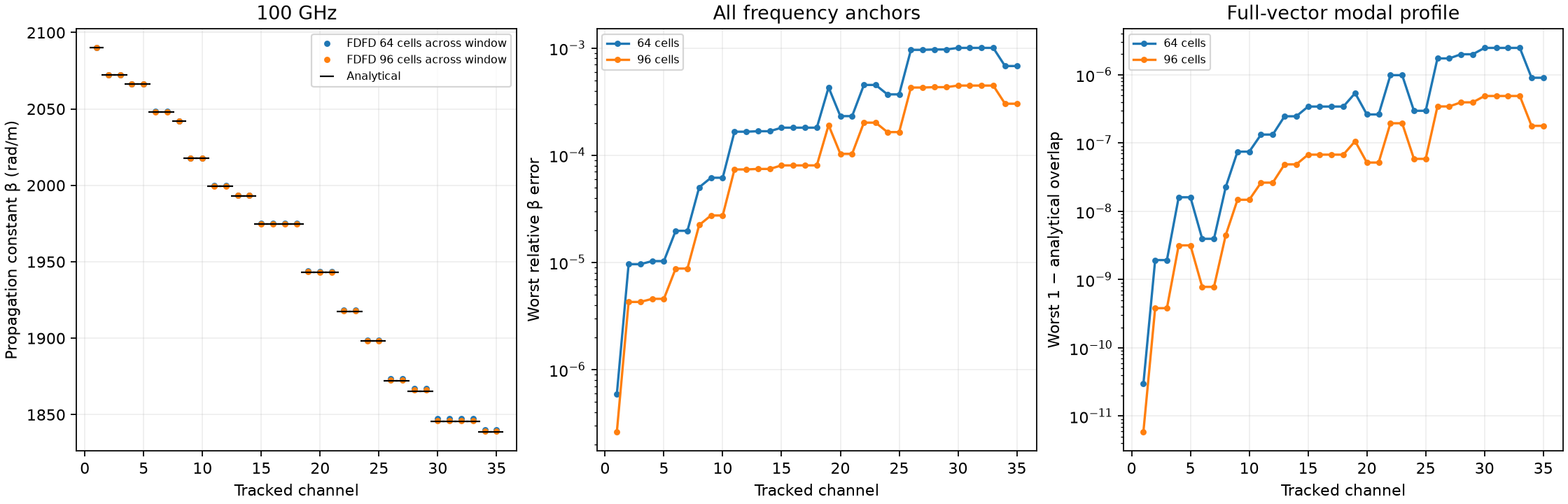
Fig. 22 C2v rectangle 2to1 PEC: comparison.

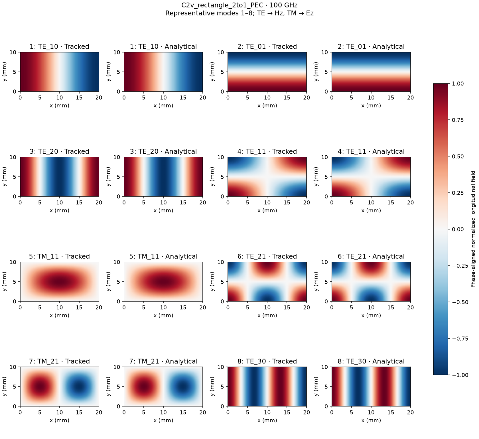
Fig. 23 C2v rectangle 2to1 PEC: modal profiles 1.

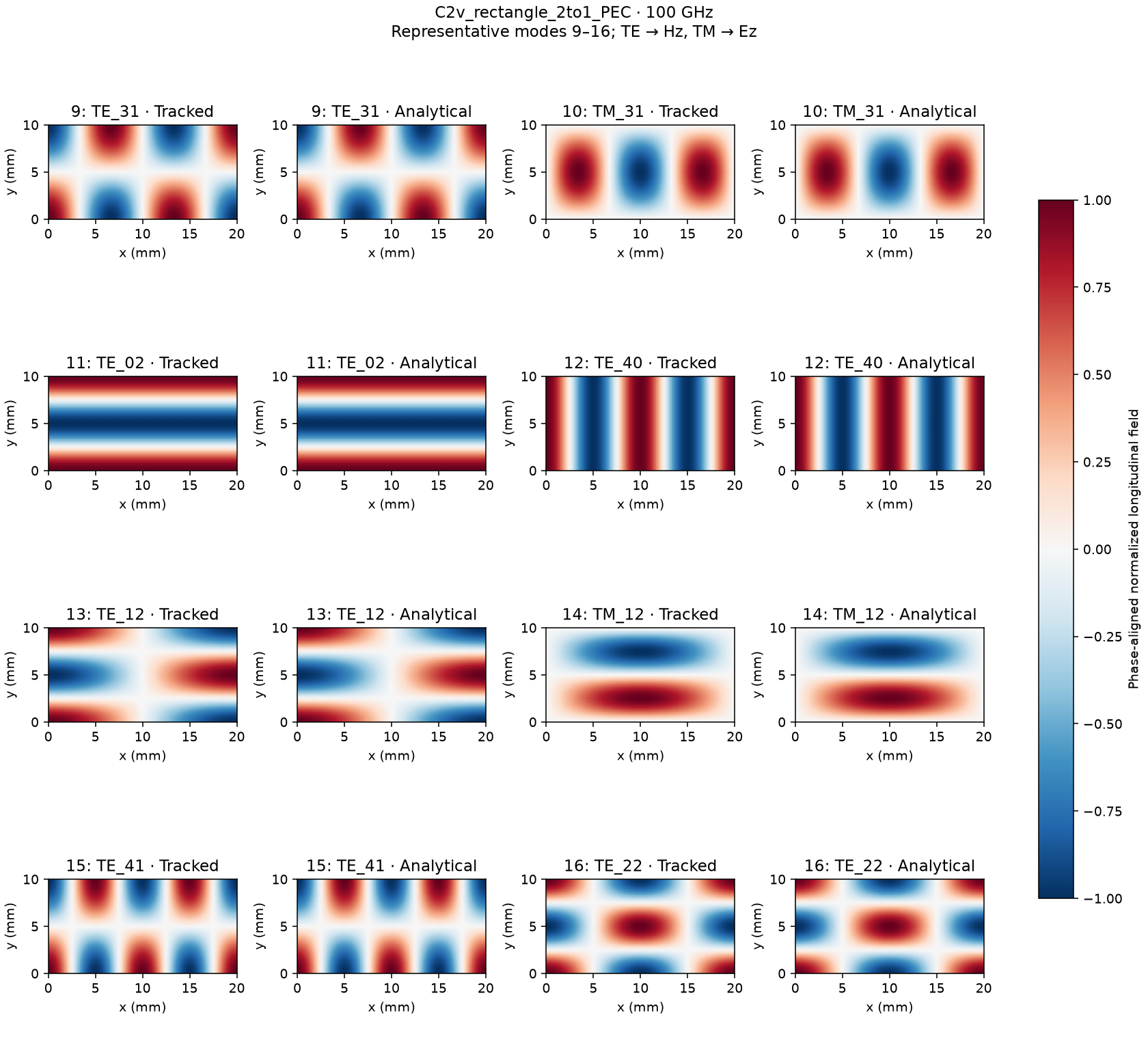
Fig. 24 C2v rectangle 2to1 PEC: modal profiles 2.

C4v square PEC

Recorded results

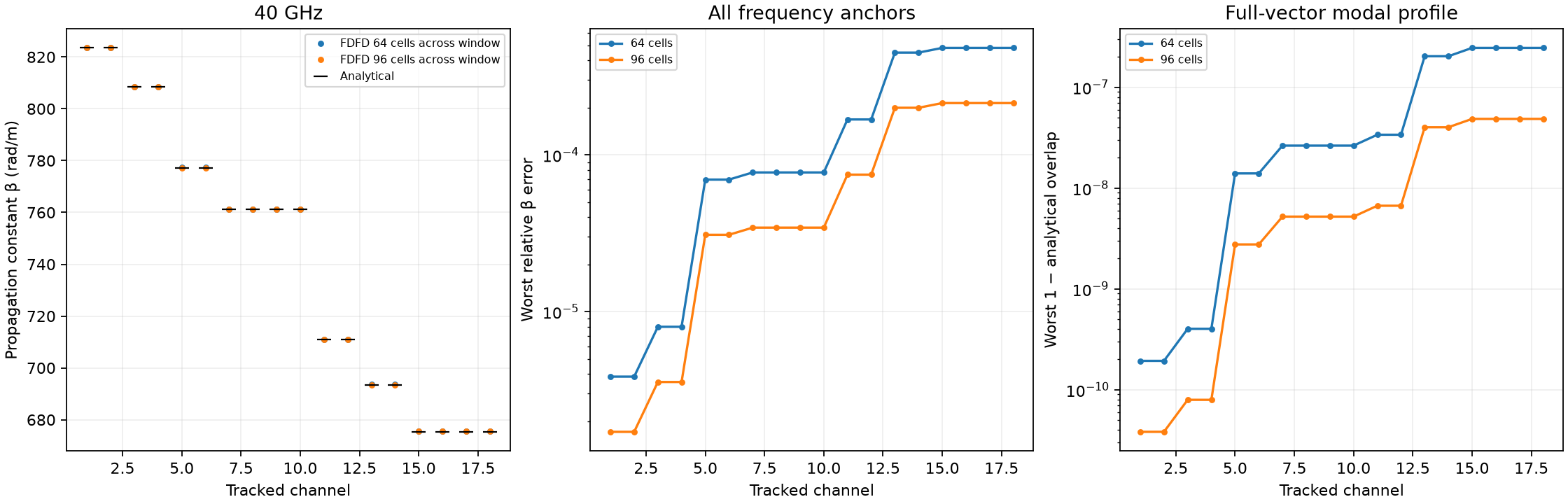
Fig. 25 C4v square PEC: comparison.

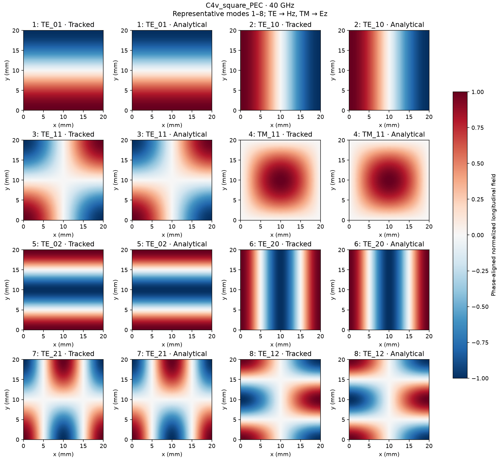
Fig. 26 C4v square PEC: modal profiles 1.

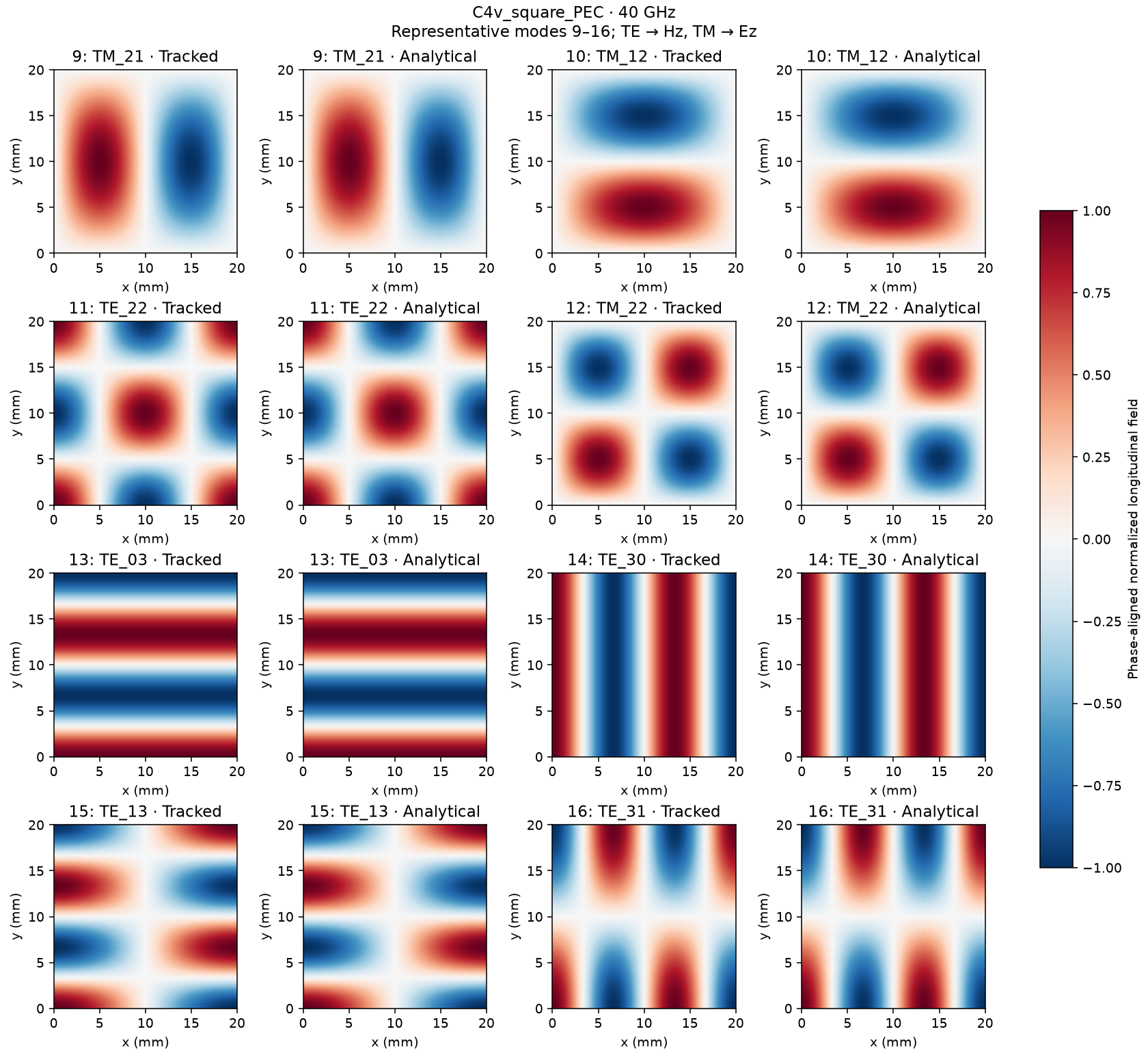
Fig. 27 C4v square PEC: modal profiles 2.

C4v cylindrical PEC

Recorded results

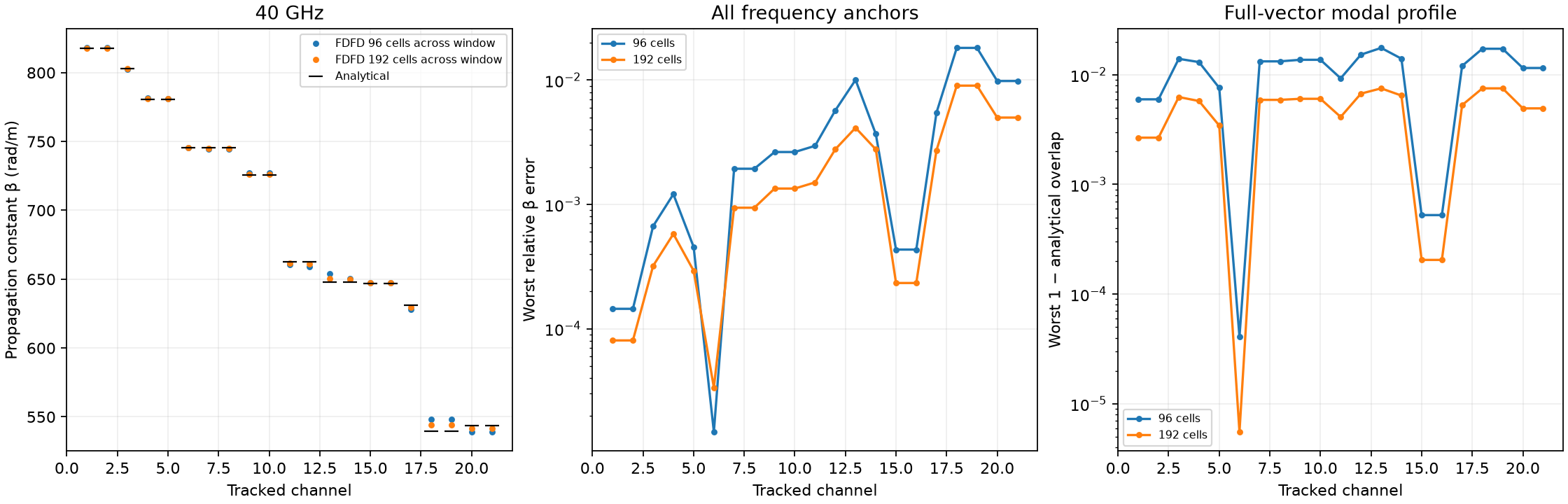
Fig. 28 C4v cylindrical PEC: comparison.

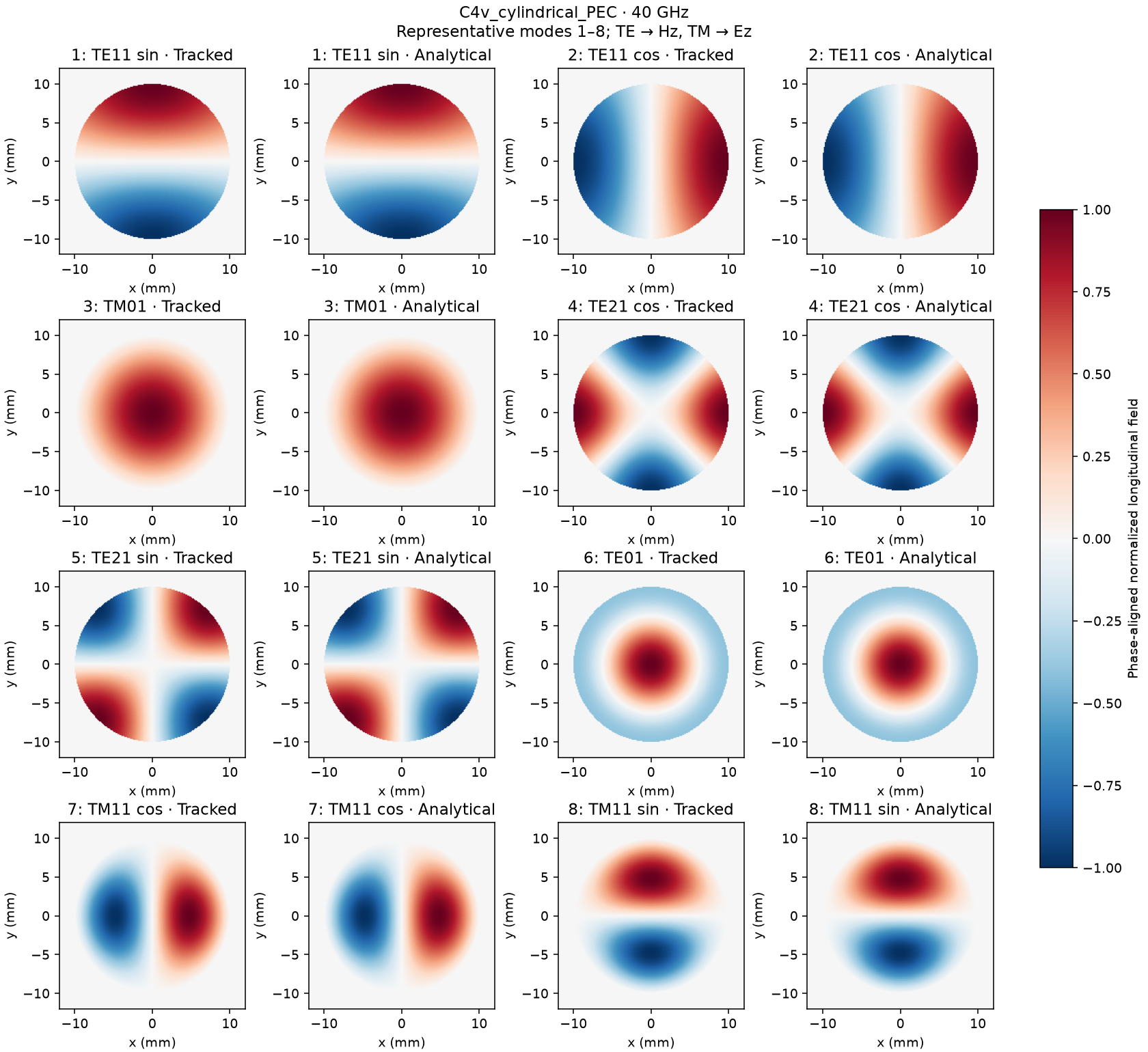
Fig. 29 C4v cylindrical PEC: modal profiles 1.

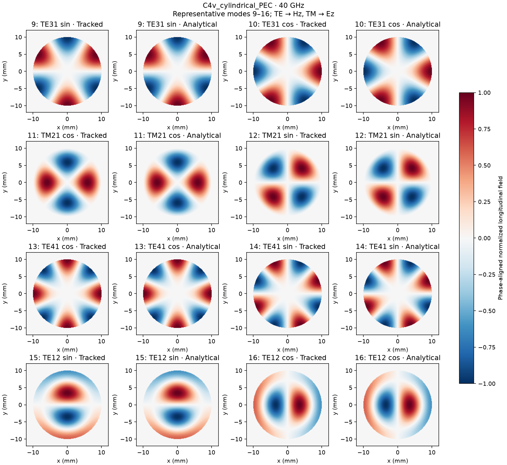
Fig. 30 C4v cylindrical PEC: modal profiles 2.

cylindrical dielectric

Recorded results

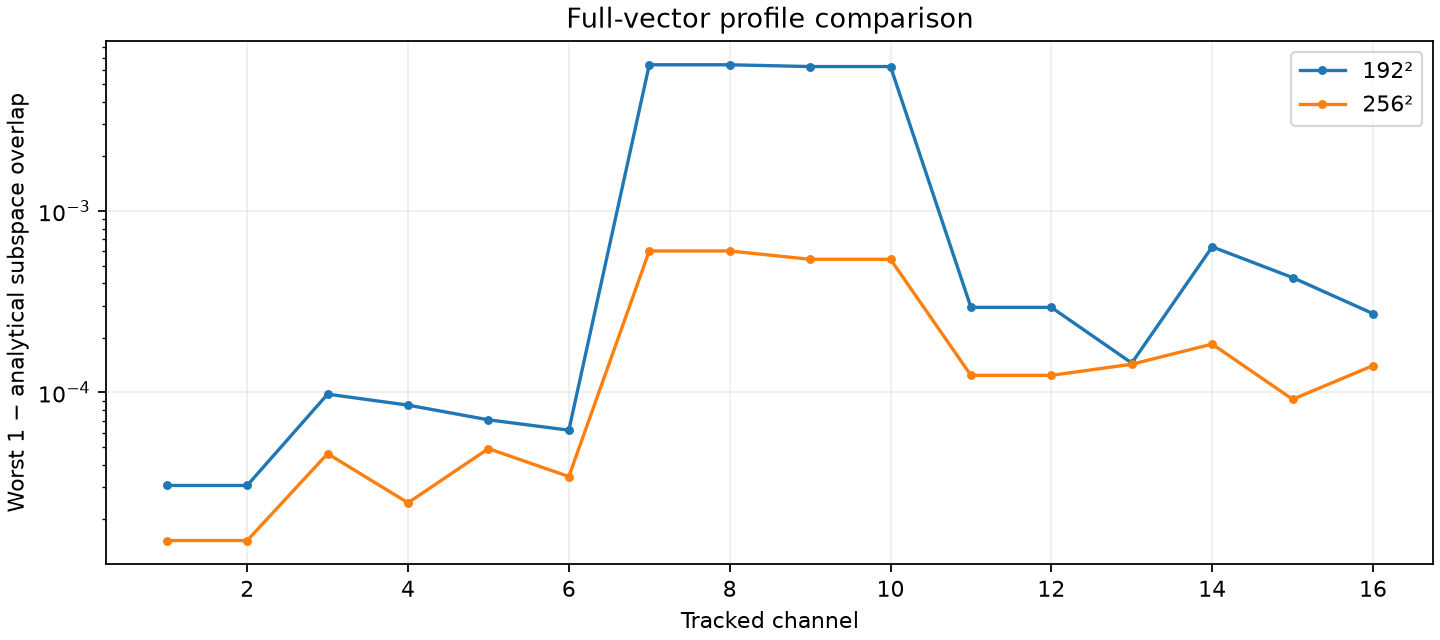
Fig. 31 cylindrical dielectric: profile matching.

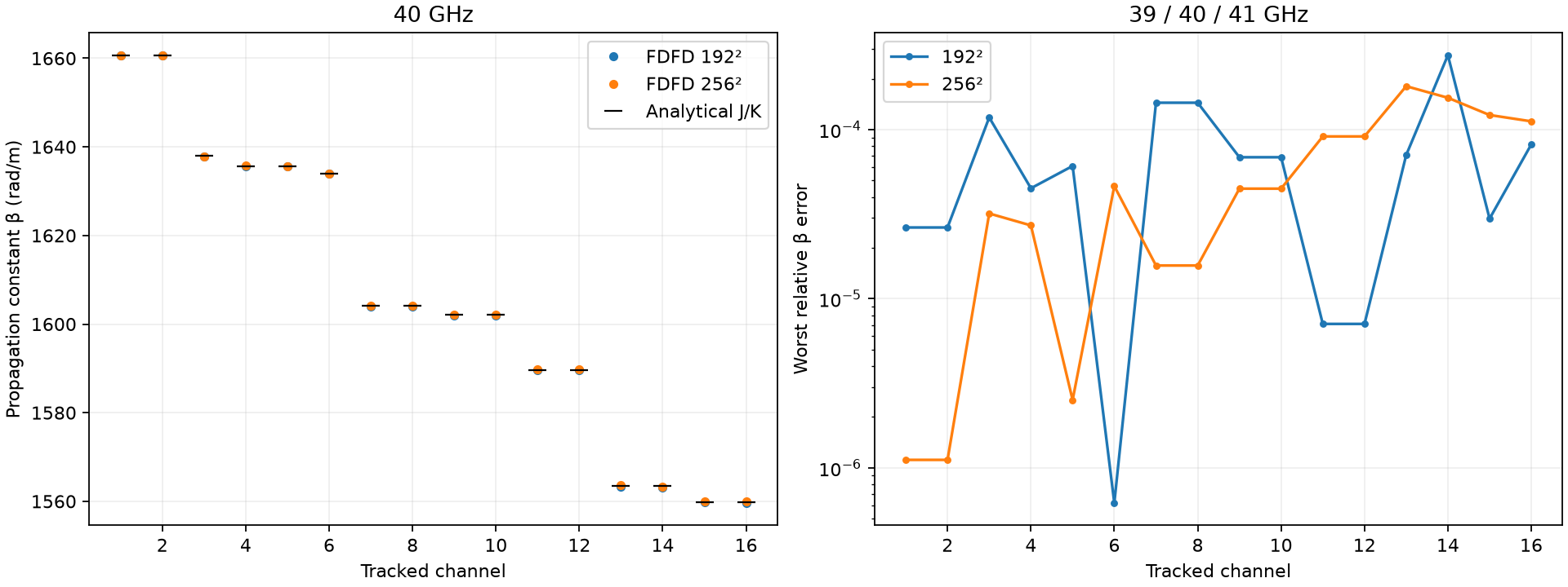
Fig. 32 cylindrical dielectric: propagation constants.

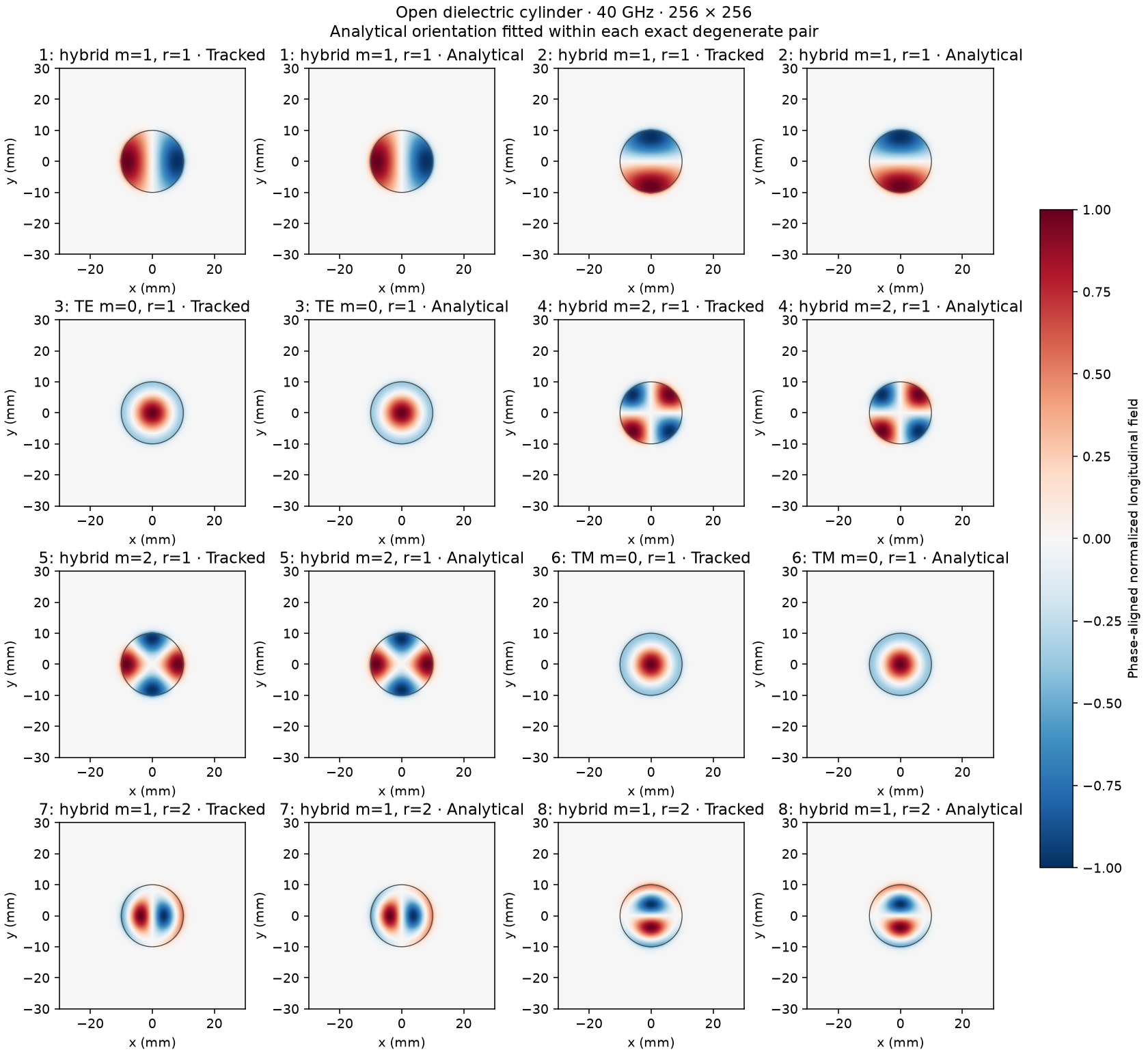
Fig. 33 cylindrical dielectric: modal profiles 1.

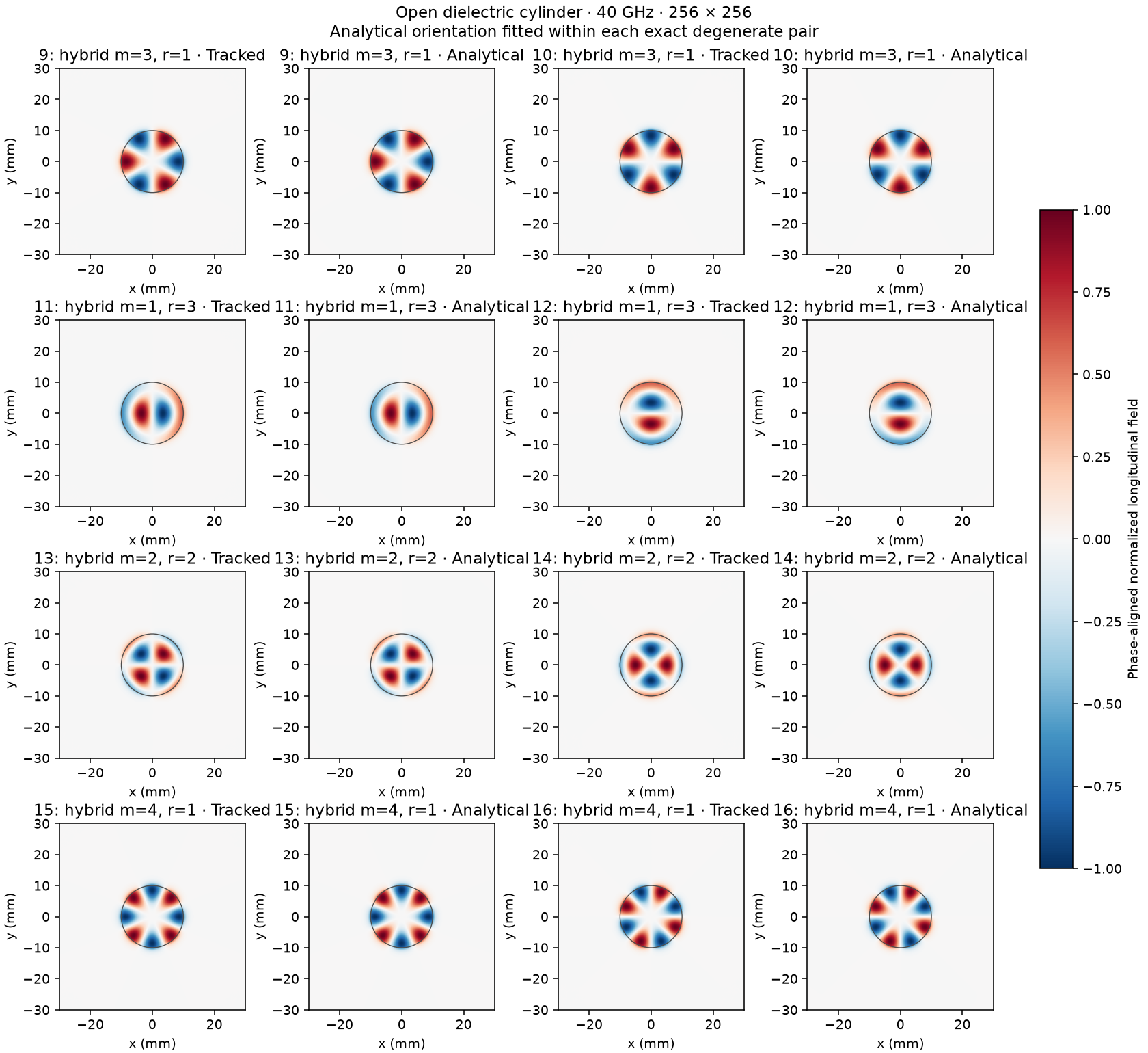
Fig. 34 cylindrical dielectric: modal profiles 2.

Branch crossing

A 20-mm square PEC bore is uniformly filled with \(\operatorname{diag}(2,2,\epsilon_z)\). At 20 GHz the sweep varies \(\epsilon_z\) from 2.3 to 2.7. This is a material-parameter sweep, not a causal dispersive frequency sweep. Independent continuum dispersion is

\[\beta_{\mathrm{TE},mn}^2=\epsilon_t k_0^2-k_{c,mn}^2, \qquad \beta_{\mathrm{TM},mn}^2=\epsilon_t k_0^2- \frac{\epsilon_t}{\epsilon_z}k_{c,mn}^2.\]

The persistent TE20/TE02 and TM12/TM21 doublets cross at \(\epsilon_z=2.5\). Tracking keeps two doublets through the coincidence and preserves their identities after raw eigenvalue ranks exchange. The exact continuum crossing and displaced finite-difference crossing are recorded separately. At each mesh’s exact numerical coincidence, all four input modes are deliberately mixed by a seeded complex unitary matrix; the tracker must recover the two persistent pairs. Fine-mesh maximum relative β error is 0.00697%, and minimum full-vector pair overlap is 0.999999992.

square anisotropic bore

Recorded results

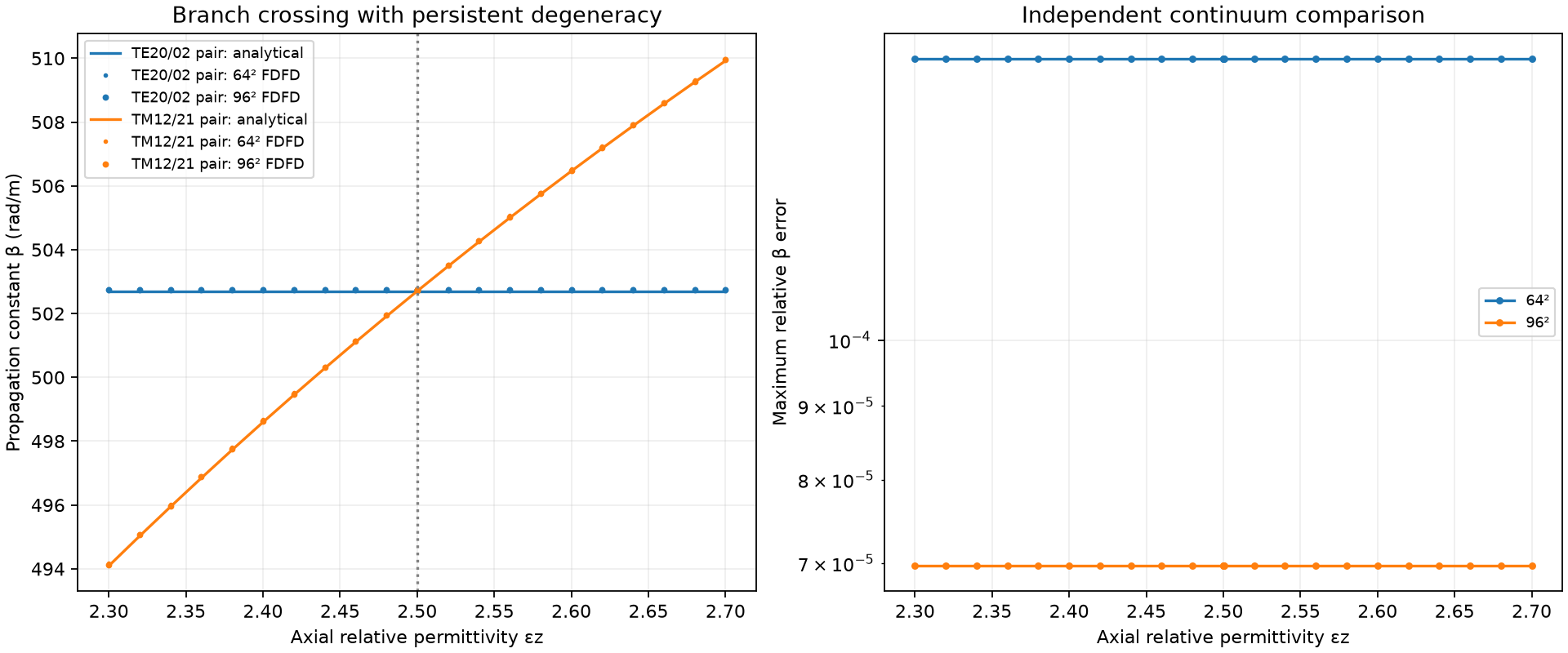
Fig. 35 square anisotropic bore: propagation constants.

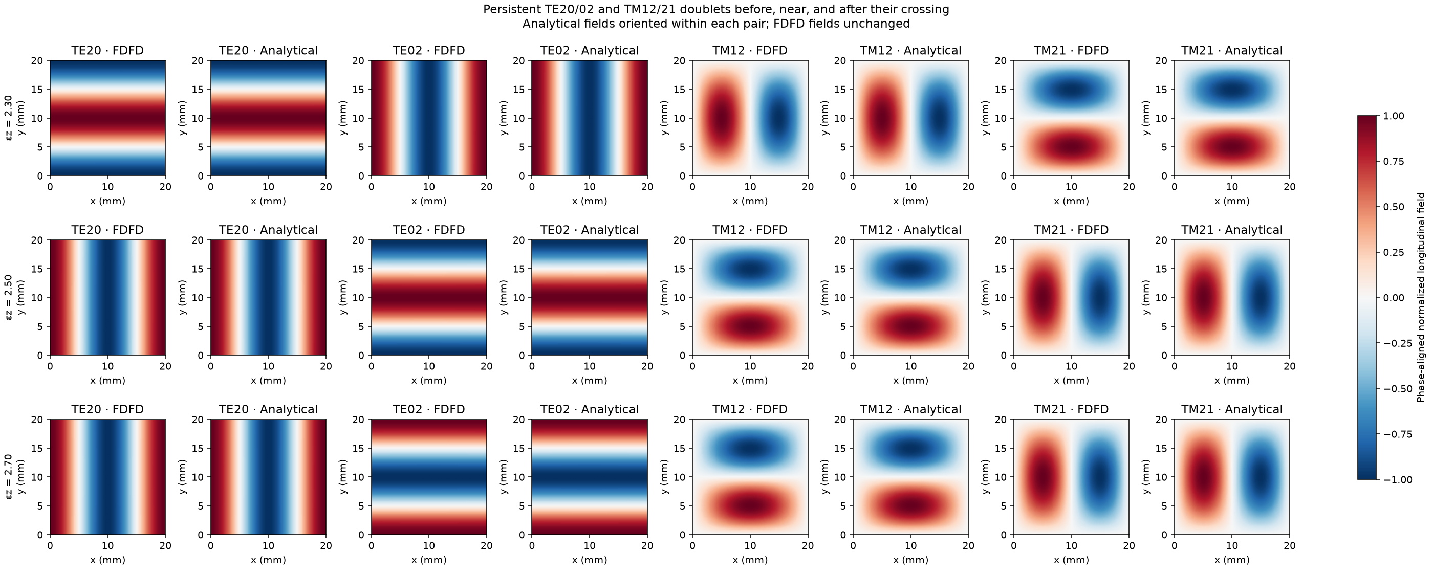
Fig. 36 square anisotropic bore: modal profiles.

Reproduce

Run from the repository root, using fresh output directories:

python -m testing.validation.eigenmode_tracking.degenerate_subspace.validate_dielectric_cylinder --output results/cylindrical_dielectric --scratch results/cylindrical_dielectric_raw
python -m testing.validation.eigenmode_tracking.branch_crossing.square_anisotropic_bore --output results/square_anisotropic_bore

Reproduce the three PEC analytical comparisons with:

python -m testing.validation.eigenmode_tracking.degenerate_subspace.validate_pec_guides --output results/pec_guides --scratch results/pec_guides_raw

plot_pec_comparison.py renders compact comparisons from a JSON report and its original field archive. Numerical regression fixtures remain under testing/eigenmode_support; they are not additional validation galleries. Check the independent analytical fields and related tracking code with:

python -m pytest tests/test_tracking_analytical_references.py tests/test_eigenmode_expanded_validation.py tests/test_waveguide_modal_profiles.py tests/test_cylindrical_modal_profiles.py