Analytical comparisons

This section compares production gprMax results with independent analytical solutions. These are correctness validations: unlike the inter-code studies, the reference is not the output of another numerical solver. Two supplementary studies in the planar-layered section are explicitly labelled as verifications: they reproduce a published benchmark or demonstrate convergence to the production NTFF result, and are not counted as independent analytical evidence.

Two levels are provided. Compact tests in tests/ntff exercise the complete FDTD and near-to-far-field path during routine pytest runs. The higher resolution studies in testing/validation are deliberately run manually; they write plots, CSV data, a machine-readable summary, and a report containing the numerical acceptance checks. The large HDF5 solver files are reproducible working data and are not the analytical reference.

TE10 transmission across cutoff

The partial-cutoff rectangular-waveguide model compares the generalized TE10 transmission coefficient with

\[S_{21}(f) = \exp[-j\beta(f)L],\]

where the two modal reference planes are separated by \(L=12\) mm. Below cutoff, \(\beta=-j\alpha\), so the field-amplitude magnitude decays as \(\exp(-\alpha L)\) and its phase is zero. Above cutoff, the ideal magnitude is 0 dB and the unwrapped phase is \(-\beta L\).

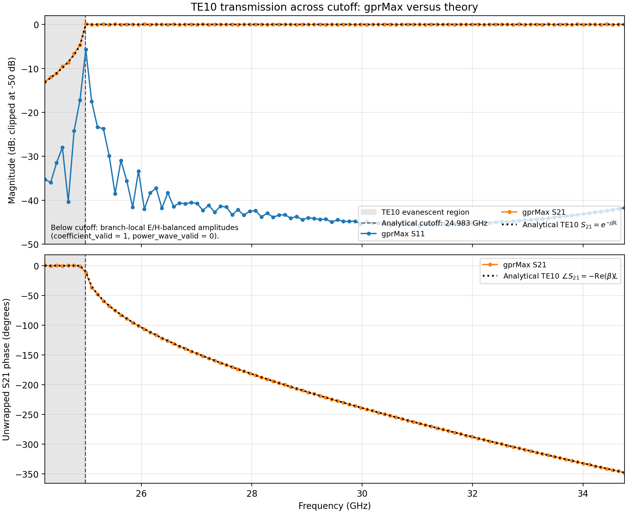
Fig. 86 gprMax and analytical TE10 transmission magnitude and phase across cutoff. The shaded below-cutoff coefficients are generalized modal amplitudes, not physical power waves.

The retained 100-frequency result has maximum theory errors of 0.353 dB in magnitude and 2.145 degrees in phase. Seven samples lie below cutoff and remain finite generalized coefficients while their separate power-wave-valid flags are false. The comparison uses the integrated eigenmode-port result directly; it does not use auxiliary receiver-derived oracle traces.

Full incident-matrix modal de-embedding

An eigenmode study records every port’s incident and outgoing modal waves in every independent excitation case. With those case vectors as columns,

\[A=[a^{(1)}\;\cdots\;a^{(N)}], \qquad B=[b^{(1)}\;\cdots\;b^{(N)}], \qquad B=SA.\]

The multiport validation driver first prescribes an exact frequency-dependent \(S\) and a non-diagonal \(A\), then forms \(B\) analytically. The production conditioned solve recovers \(S\) with a maximum Frobenius-norm error of \(4.61\times10^{-16}\). Dividing each case only by its nominal source wave has an error of at least \(2.17\times10^{-2}\) in this test.

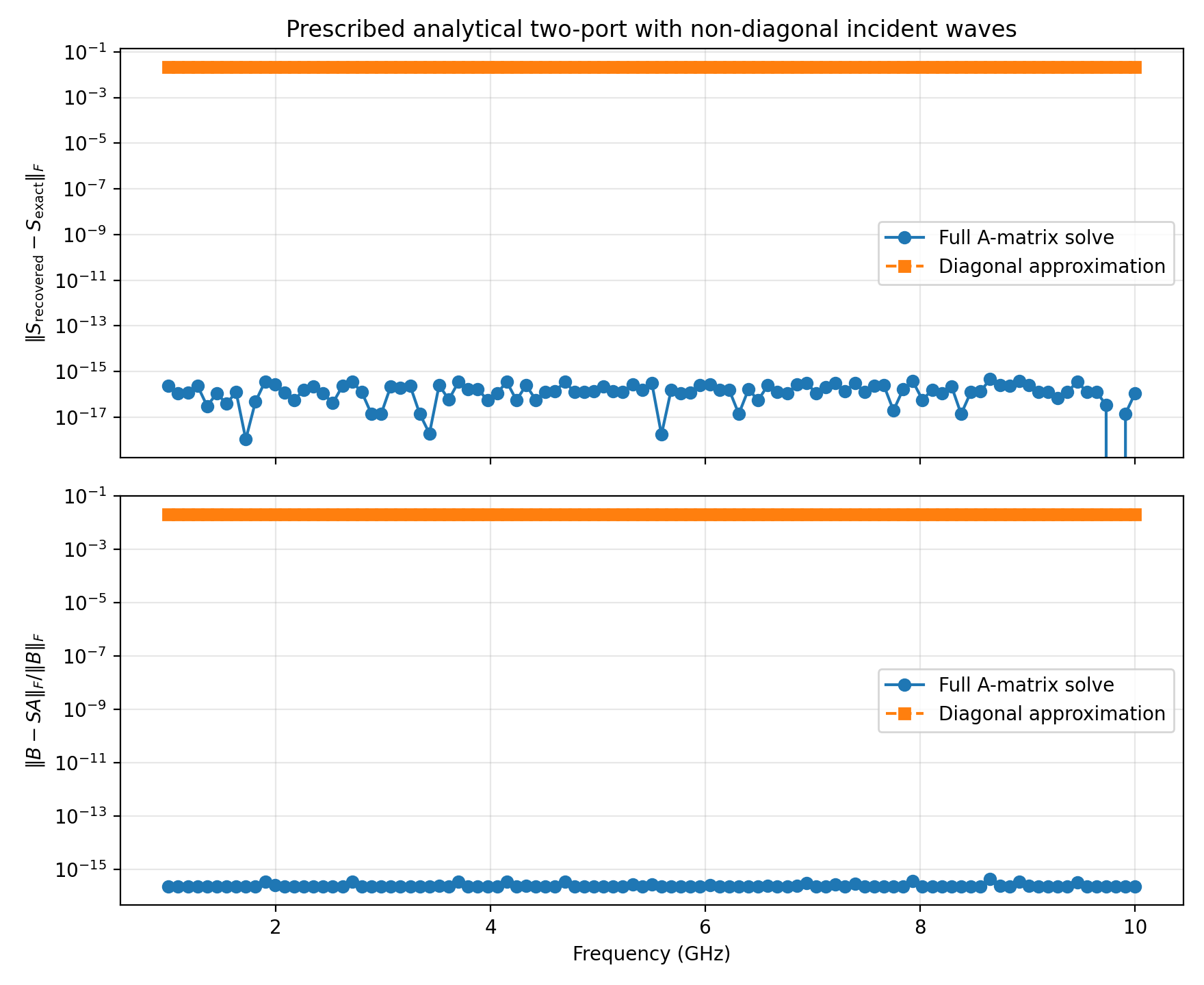
Fig. 87 Exact matrix recovery and network-equation residual with deliberately non-zero incident waves at nominally passive ports.

The end-to-end comparison uses a lossless two-port rectangular guide and the analytical TE10 propagation factor \(\exp(-j\beta L)\). Across 20–24 GHz, the full solve has maximum errors of 0.002037 in linear magnitude and 1.226 degrees in phase. Its maximum \(\|B-SA\|/\|B\|\) residual is \(3.70\times10^{-16}\), compared with 0.0399 for diagonal normalisation.

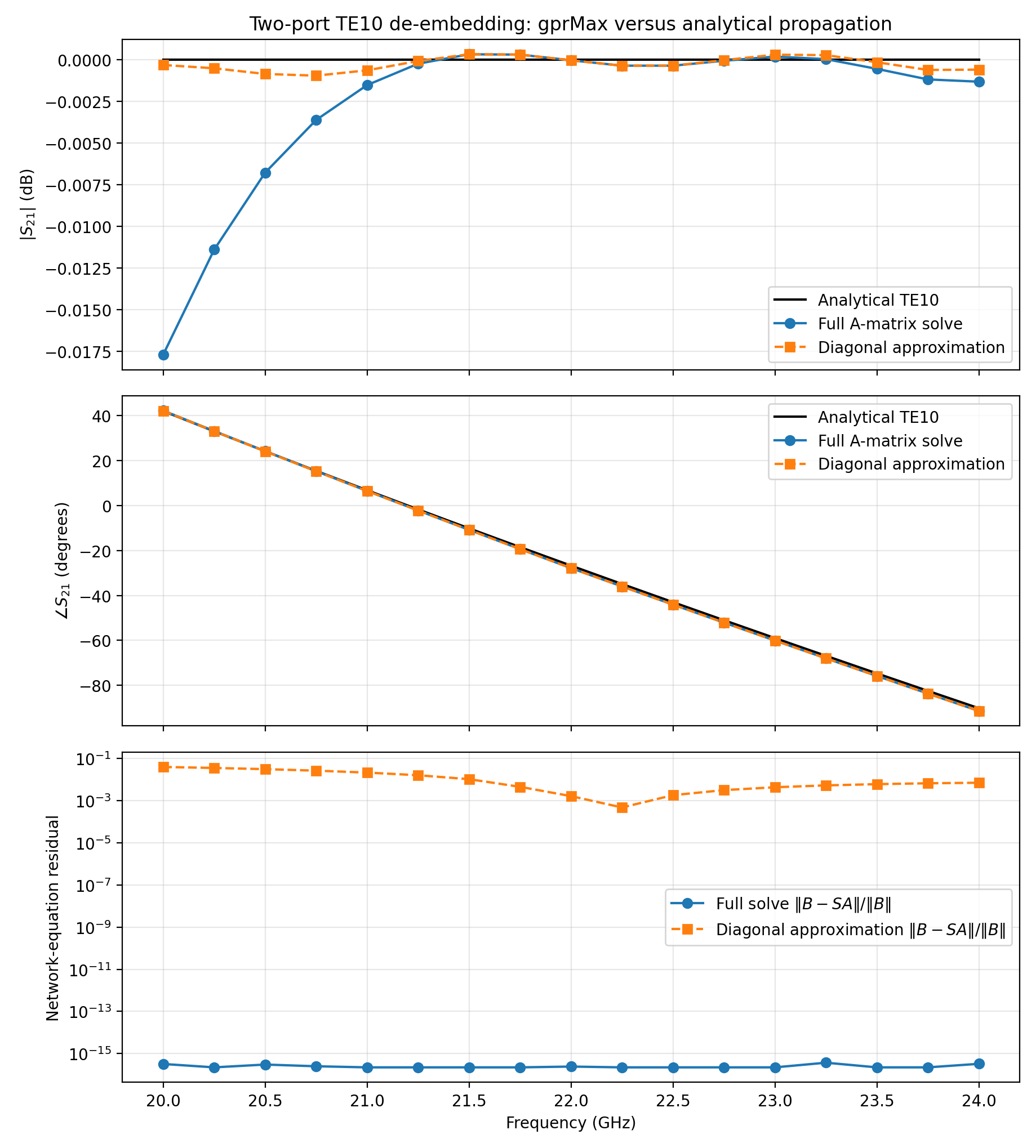
Fig. 88 End-to-end TE10 comparison and the measured multiport network residual. The diagonal result is accidentally closer to the continuum magnitude in this coarse model, but it does not satisfy the measured \(B=SA\) system; full de-embedding does not remove ordinary FDTD discretisation or port-termination errors.

Hertzian dipole in free space

hertzian_dipole_fs_analytical.in

This example is a Hertzian electric dipole, i.e. an additive electric-current source, in free space.

#title: Hertzian dipole in free-space
#domain: 0.100 0.100 0.100
#dx_dy_dz: 0.001 0.001 0.001
#time_window: 3e-9

#waveform: gaussianprime 1 1e9 myWave
#hertzian_dipole: z 0.050 0.050 0.050 myWave
#rx: 0.070 0.070 0.070

The function hertzian_dipole_fs in testing/analytical_solutions.py evaluates the complete free-space time-domain solution at the Yee-component positions. The relative source and receiver positions are important because the six field components are spatially staggered.

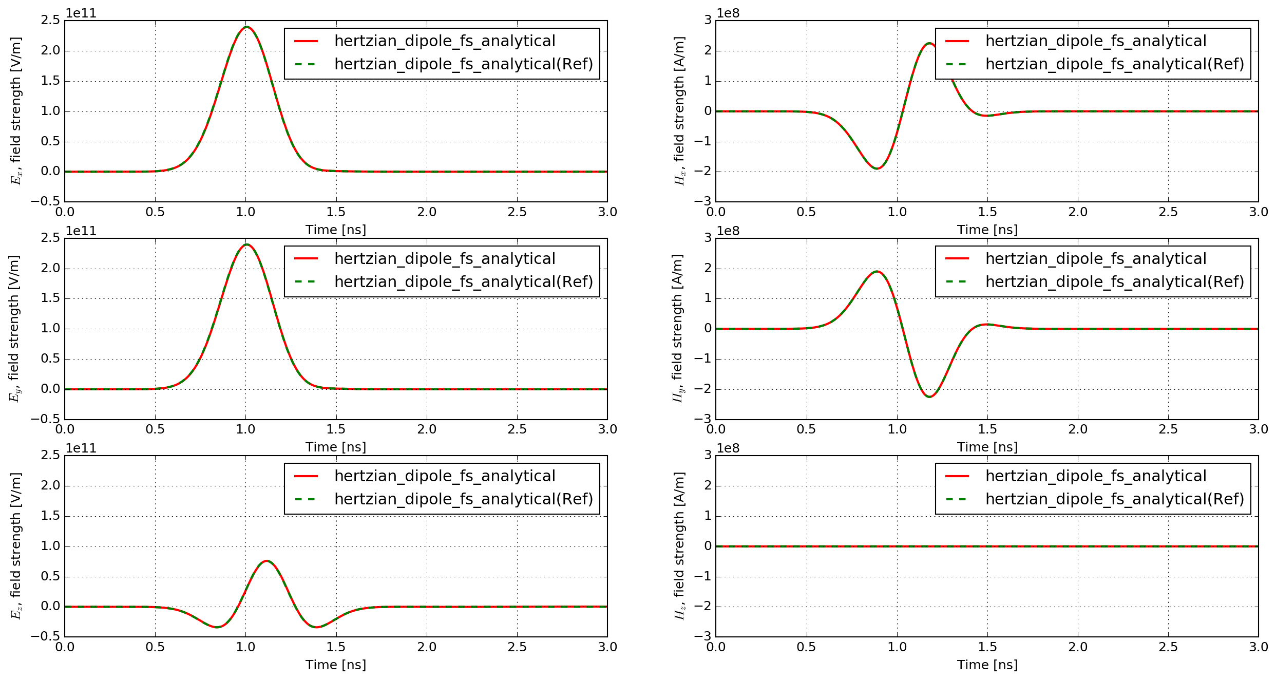
Fig. 89 Electric and magnetic field histories from gprMax and the analytical solution (Ref).

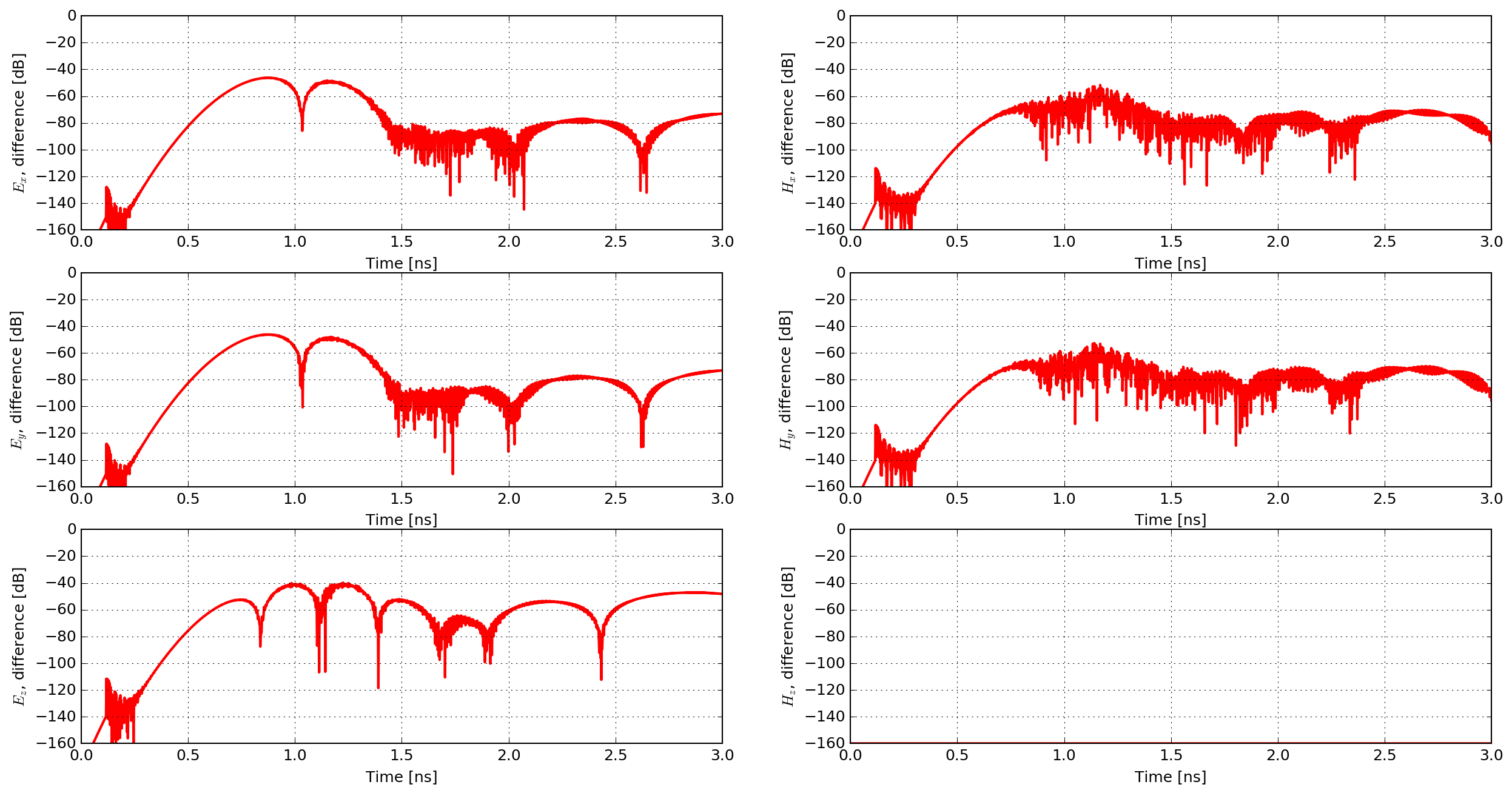
Fig. 90 Percentage differences between the numerical and analytical fields.

The largest difference is approximately one percent in the electric component parallel to the source. The remaining electric components are within about 0.5 percent and the magnetic components within about 0.25 percent.

Plane-wave reflection from dispersive half spaces

The normal-incidence validation calculates the incident waveform in free space, repeats the model with a planar half space, and obtains the reflected field by subtraction. The complex reflection coefficient is compared with the Fresnel result

\[\Gamma(\omega) = \frac{\eta_2(\omega)-\eta_1(\omega)} {\eta_2(\omega)+\eta_1(\omega)},\]

where the frequency-dependent wave impedance is evaluated from the same dielectric, conductivity, Debye, Lorentz, or Drude parameters used to define the material. Propagation phase between the receiver and the effective Yee interface is included explicitly.

Dispersive half-space driver tests a nondispersive dielectric, one- and three-pole Debye media, and multi-pole Lorentz and Drude media over 0.25–8 GHz.

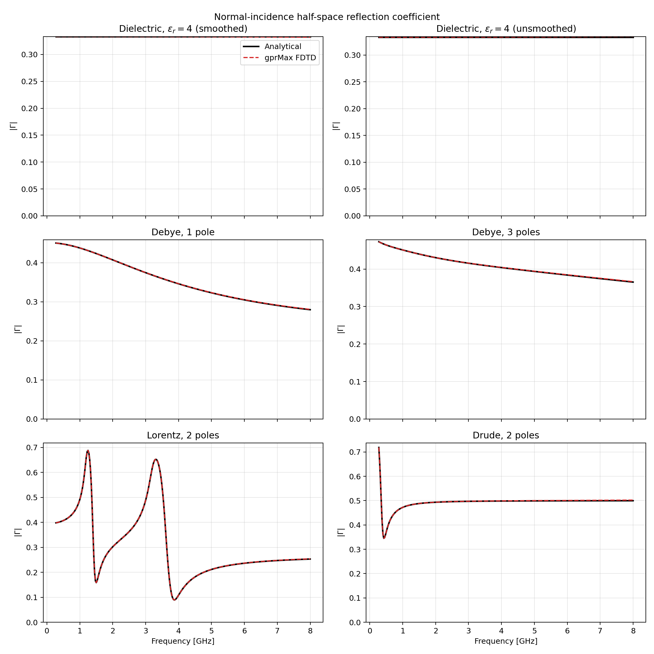
Fig. 91 Magnitude of the gprMax reflection coefficients and the corresponding Fresnel solutions.

Across the retained result set, magnitude RMS errors are between \(3.3\times10^{-4}\) and \(1.2\times10^{-3}\). The maximum phase RMS error is 0.021 degrees. These comparisons exercise the discrete plane-wave source and the complete multipole material-update path, rather than only evaluating the material formula in isolation.

Realistic-material driver adds fresh water at 25 degrees Celsius and Puerto Rico clay with ten percent volumetric water content over frequency ranges selected to show their dispersion.

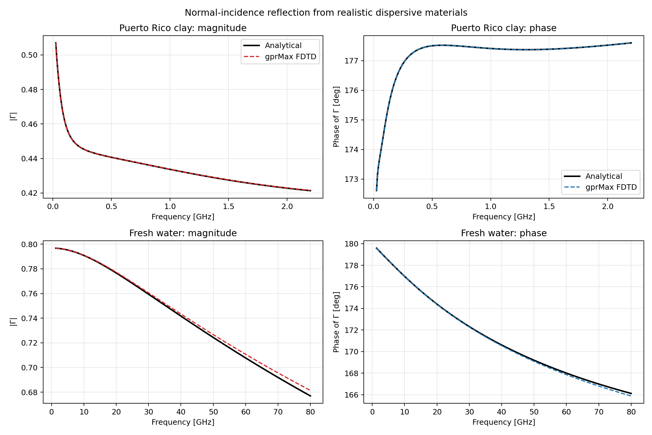
Fig. 92 Complex Fresnel comparison for the fresh-water and clay models.

Planar-layered near-to-far-field transform

The planar-layered NTFF validation driver places a z-directed Hertzian current element in a finite lossy, magnetic film between two lossless half-spaces. The closed Huygens surface crosses both interfaces, so a homogeneous-background transform is not applicable. The production surface result is compared with the independent three-layer transmission-line Green function of Çapoğlu et al. [CAP2012].

For a dipole current moment \(\widetilde p(\omega)\) in layer \(n\), the range-normalised analytical field is

\[r e^{+j k_o r} E_\theta =s\,\frac{j\omega\mu_o}{4\pi}\, \widetilde p(\omega) V_{v_n}^{\mathrm{TM}}(z_0) \frac{\epsilon_o}{\epsilon_n}\sin\theta,\]

where \(s=+1\) and \(-1\) for observation in the positive- and negative-axis exterior respectively. The voltage-source response \(V_{v_n}^{\mathrm{TM}}\) is evaluated from the closed three-layer form, independently of the production surface integration. The exact discrete Hertzian-source samples and their Yee time offset are read from the output, so waveform amplitude and phase are not fitted.

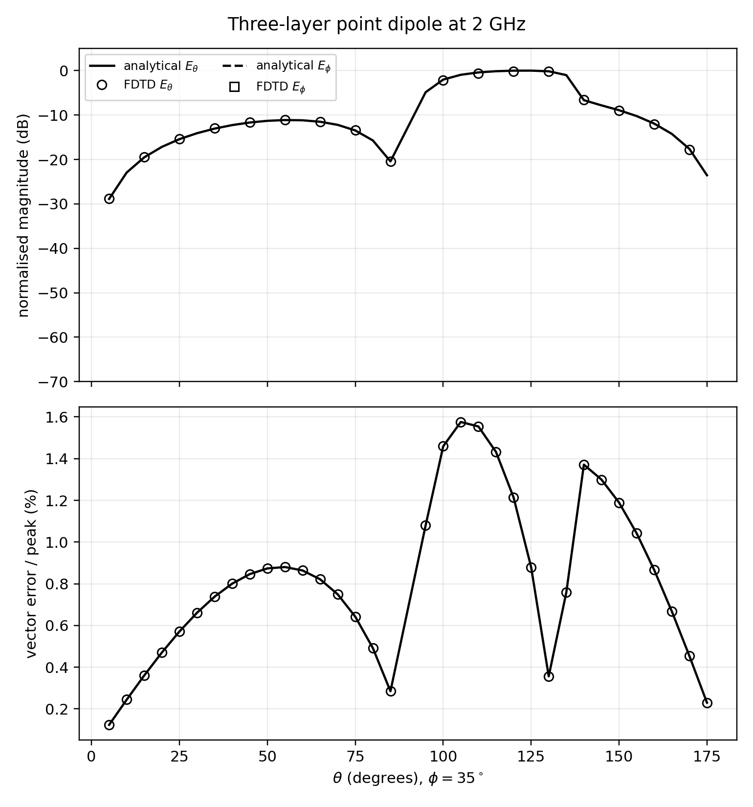
Fig. 93 FDTD Huygens-surface result (symbols) and the analytical three-layer point-dipole field (lines) across both observation half-spaces.

The retained 1 mm result spans nine frequencies from 1–3 GHz. Its maximum vector error normalised to the analytical peak is 2.304 percent and its RMS error is 0.857 percent. Repeating the model at 2 mm gives 4.738 and 1.722 percent, respectively, demonstrating the expected improvement under mesh refinement. The comparison exercises the complete field collection, Yee-time correction, material-interface smoothing, complex TE/TM recursion, and angular far-field evaluation.

Grounded-slab direct-time benchmark

The grounded-slab validation driver reproduces Figure 11 of Çapoğlu’s thesis [CAP2007]. Horizontal and vertical Hertzian electric dipoles lie 1 mm below the air interface of a 2 mm, \(\epsilon_r=2.5\) slab backed by a PEC plane. The spatial step is the published 0.1 mm, the differentiated-Gaussian pulse has \(\tau=5\) ps, and \(rE_\theta\) is observed at \(\theta=\phi=45\) degrees. The analytical curves in the thesis were obtained from Cicchetti’s grounded-slab expressions [CIC1993].

For either TE or TM polarisation \(p\), the independent validation uses the grounded echo train

\[V^p(t)=\sum_{n=0}^{\infty} \Upsilon^p_{10}(-\Gamma^p_{10})^n \delta\!\left(t-\frac{2nh}{v_1}\right),\]

and the source-in-slab voltage and current responses

\[V_v^p(t\mid z')=\frac{1}{2} \left[V^p\!\left(t+\frac{z'}{v_1}\right) +V^p\!\left(t-\frac{2h+z'}{v_1}\right)\right],\]

\[V_i^p(t\mid z')=\frac{Z_1^p}{2} \left[V^p\!\left(t+\frac{z'}{v_1}\right) -V^p\!\left(t-\frac{2h+z'}{v_1}\right)\right].\]

These are Eqs. (59), (63), and (65) of [CAP2007]. The validation evaluates the series independently, uses the stored half-step current samples, and places the point current at the centre of its Yee edge. Neither amplitude, phase, nor time is fitted. A common source pre-delay is removed from the reported axis; it only places the published pulse inside the transform’s complete retarded-history interval.

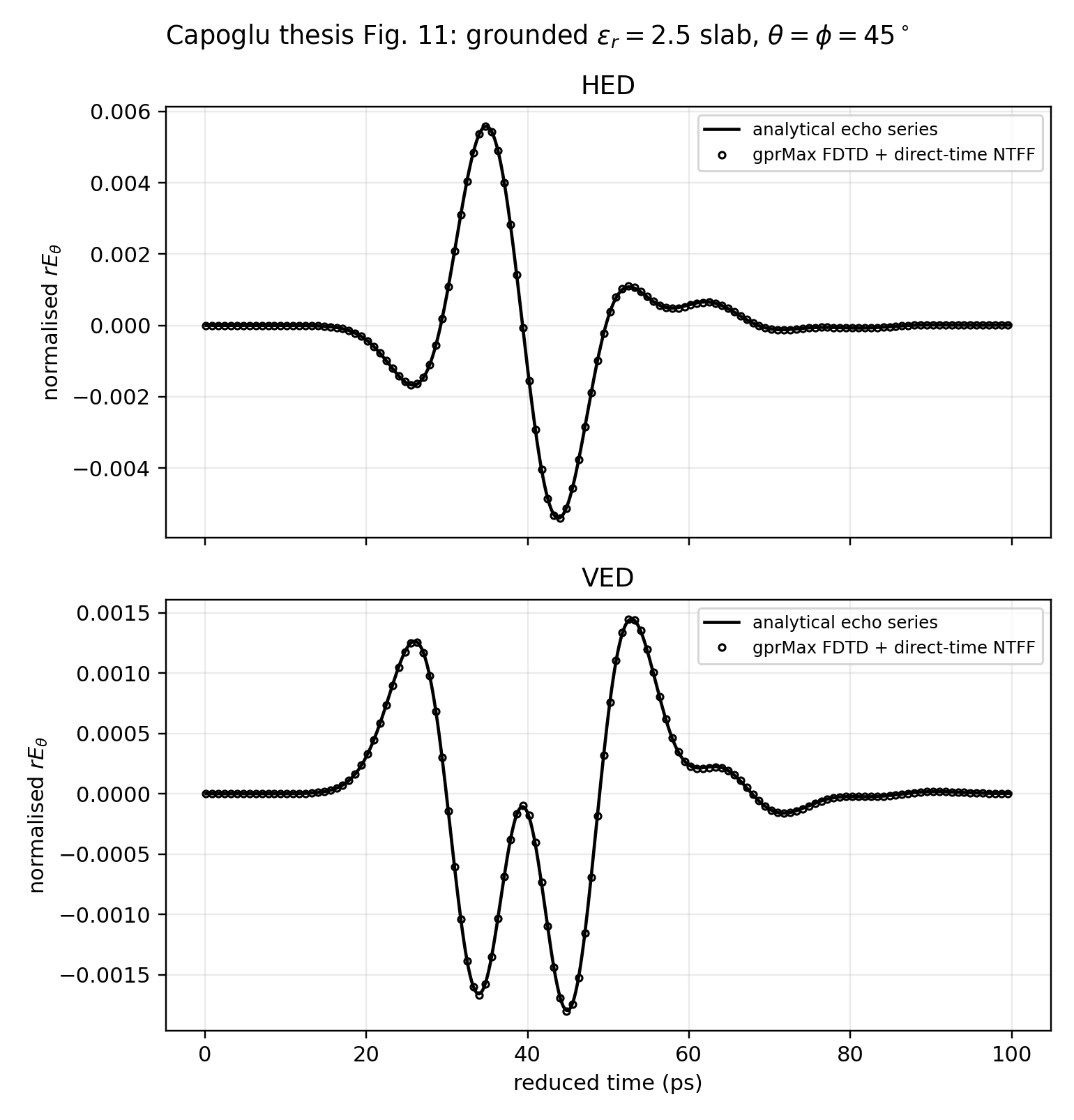
Fig. 94 Published grounded-slab HED and VED configurations: the independent echo series is shown by lines and the gprMax FDTD/direct-time transform by symbols.

The HED maximum and RMS errors are 0.494 and 0.149 percent of the analytical peak. The VED values are 0.915 and 0.287 percent. The comparison exercises the PEC short-circuit response, the five-face surface whose omitted face coincides with the ground, both tangential and normal electric-current orientations, and the complete time-domain surface transformation.

PEC image theory and coated-ground far fields

Two further drivers validate PEC termination without using curves digitised from the thesis. The grounded-dipole driver uses exact image theory for tangential and normal electric and magnetic dipoles above a bare PEC. It also places electric dipoles above a lossless \(\epsilon_r=4\) coating backed by PEC. For the coated conductor, the independent far-zone reference decomposes the dipole spectrum into oblique TM and TE plane waves. With

\[q=\sqrt{\epsilon_r-\sin^2\theta},\qquad Z_1^{\mathrm{TM}}=\eta_0\frac{q}{\epsilon_r},\qquad Z_1^{\mathrm{TE}}=\eta_0\frac{1}{q},\]

the short-circuited slab input impedance and tangential-electric-field reflection coefficient are

\[Z_{\mathrm{in}}^p=jZ_1^p\tan(k_0qd),\qquad \Gamma^p=\frac{Z_{\mathrm{in}}^p-Z_0^p} {Z_{\mathrm{in}}^p+Z_0^p}.\]

For a bare PEC, \(\Gamma^{\mathrm{TM}}= \Gamma^{\mathrm{TE}}=-1\), recovering the electric and magnetic image signs. The direct and reflected vector fields retain the physical Yee-component centre, the selected transform origin, and their separate propagation phases. This is the radiative far-zone term of the coated-conductor spectrum described by Tang and Hong [TANG2002]; finite-distance surface and lateral waves are not part of an asymptotic NTFF output.

The source location is the physical Yee-component centre, not its integer grid anchor. Electric dipoles have a half-cell shift along their polarisation axis; magnetic dipoles have half-cell shifts along the two transverse axes. For example, an x-polarised magnetic source is located at \((i\Delta x,(j+1/2)\Delta y,(k+1/2)\Delta z)\).

An absolute comparison uses the recorded source samples and their time offset \(t_0\):

\[\widehat{s}(f)=\Delta t\sum_n s_n \exp[-j2\pi f(n\Delta t+t_0)].\]

The recorded spatial scale converts this spectrum to the source moment. For the electric transverse projection and magnetic cross product used in the driver, the range-normalised far-field factors are, respectively,

\[C_E=-\frac{jk_0\eta_0}{4\pi}\widehat{I\ell},\qquad C_H=+\frac{jk_0}{4\pi}\widehat{M}.\]

Here \(\widehat{M}\) is the magnetic-current moment implied by the magnetic-dipole source update, and the time convention is \(\exp(+j\omega t)\). No amplitude or phase is fitted in this absolute comparison. A separate pattern-shape diagnostic retains the original single complex fit shared by both principal planes.

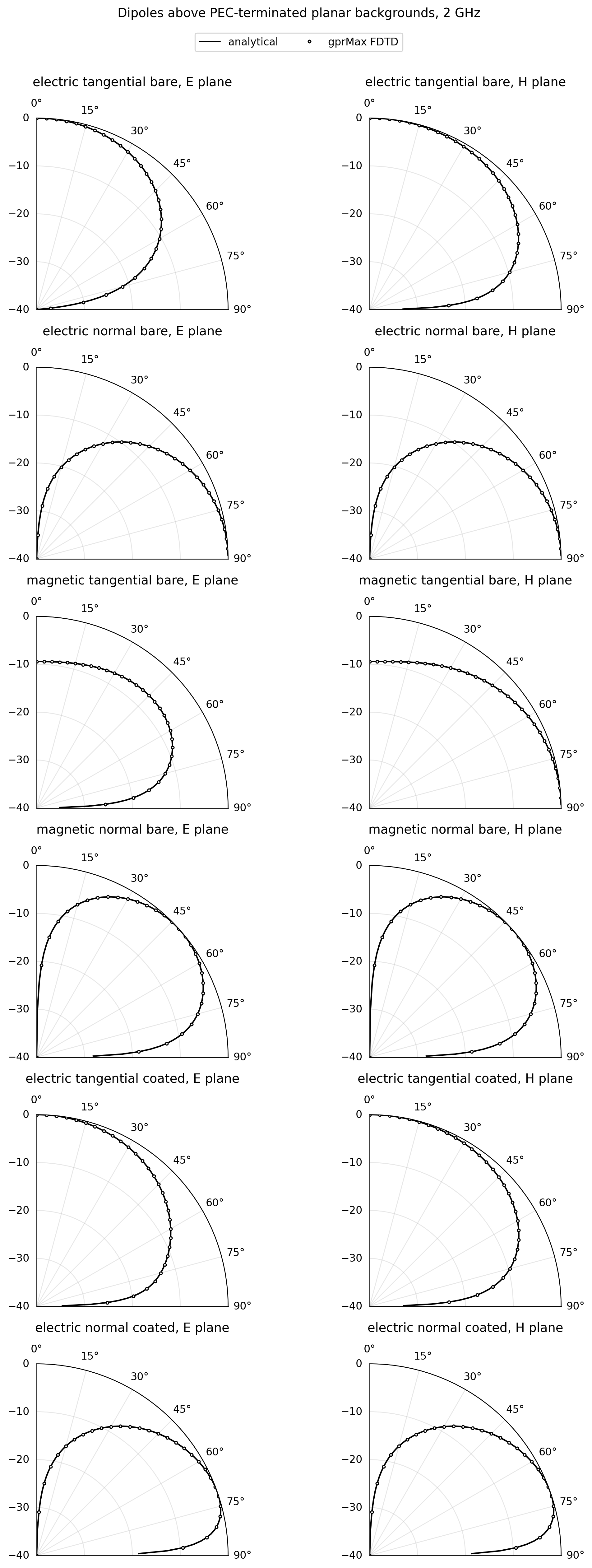
Fig. 95 Principal-plane power patterns at 2 GHz. Lines are the independent image or short-circuited-slab solution and symbols are the five-face production Huygens transform.

At 1.5 mm resolution, the worst absolute complex-vector relative L2 error over 1.5, 2.0, and 2.5 GHz is 0.04390 percent for the four bare-PEC cases and 0.13149 percent for the two coated cases. The tangential and normal magnetic bare-PEC cases give 0.01008 and 0.02717 percent, respectively. The L2 norm includes both Etheta and Ephi in both principal planes; these values are not maximum pointwise errors. The corresponding worst maximum-directivity differences are 0.09916 percent for bare PEC and 0.97664 percent for coated PEC.

Earlier larger magnetic-source discrepancies resulted from an incorrectly positioned analytical dipole, not an identified solver defect. The figures and metrics above use the corrected Yee centres. That correction alone does not establish a mesh-convergence result.

The grounded-slab reflection driver provides an independent broadband phase check. It subtracts a free-space axial-DPW trace from the total field of a 12 mm, \(\epsilon_r=4\) PEC-backed slab and de-embeds the ratio with the axial Yee numerical wavenumber.

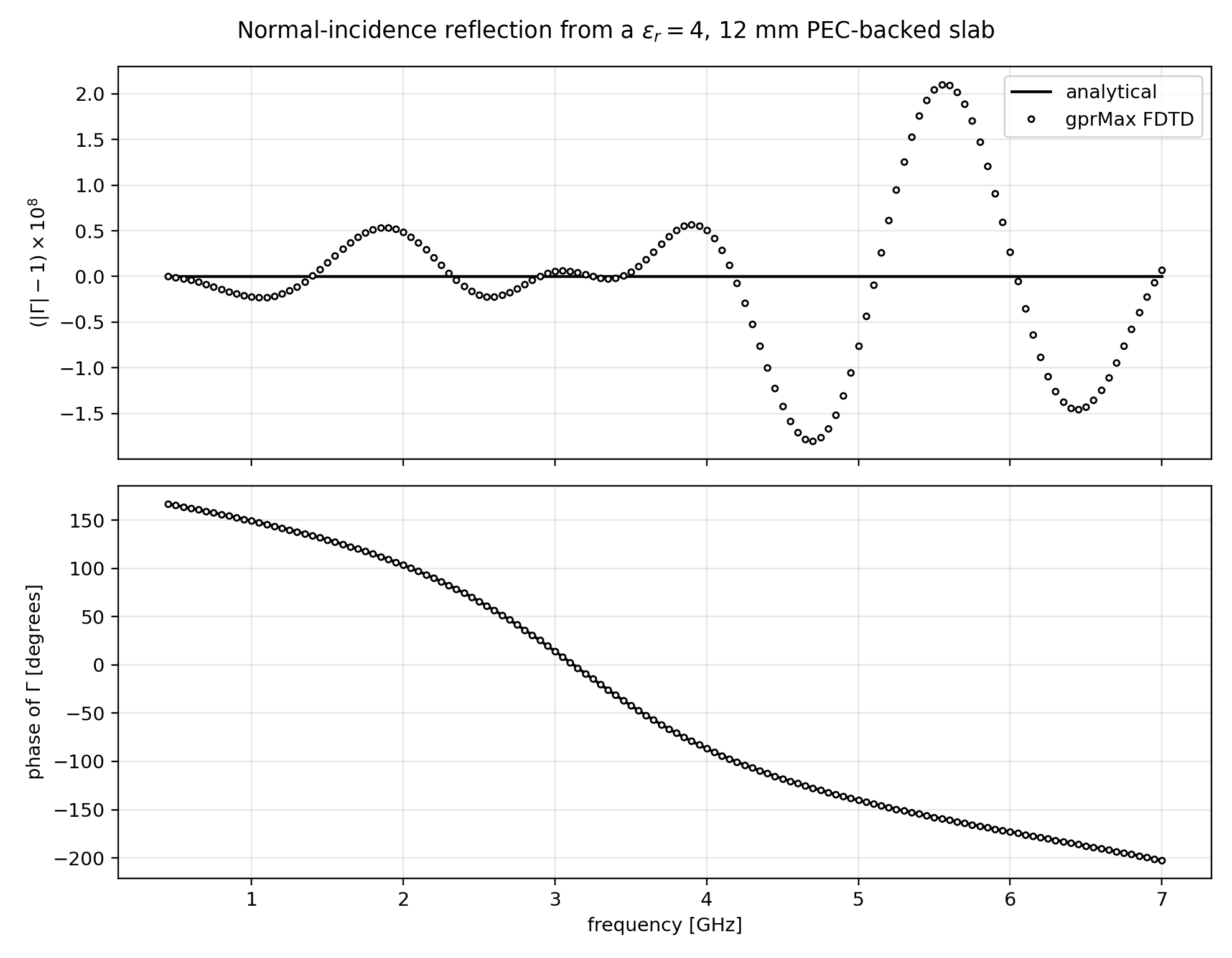
Fig. 96 Exact and FDTD complex reflection coefficient from 0.4–7.0 GHz.

Across 132 retained frequencies, the maximum magnitude error is \(2.11\times10^{-8}\), the maximum phase error is 0.0553 degrees, and the complex relative L2 error is 0.0309 percent. Normal-incidence TE and TM are degenerate in this second model; the coated-dipole E- and H-plane cuts above exercise their distinct oblique coefficients.

Published eight-layer transform verification

The Çapoğlu Figure 2 reproduction recreates the published arrangement of nine differently oriented Hertzian current elements in an eight-layer stack [CAP2012]. The relative permittivity varies from 1.3 to 1.5, relative permeability from 1.1 to 1.3, and the six finite layers are conductive. Both TE and TM terms are therefore non-zero.

For current element \(q\), the direct point-current reference has the form

\[\mathbf F_E^{\mathrm{point}}(\hat{\mathbf r},\omega) =\sum_{q=1}^{9} \overline{\overline{\mathbf G}}_E (\hat{\mathbf r},z_q,\omega)\cdot \widetilde{\mathbf p}_q(\omega) \exp\left(j\mathbf k_t\cdot\boldsymbol\rho_q\right),\]

where the layered dyadic response is evaluated in the unperturbed stack. The discrete source moments \(\widetilde{\mathbf p}_q\) and their Yee-time offsets are read from the output. They are not fitted to the NTFF result. The production result instead obtains equivalent currents from a closed surface and propagates every surface sample through the same stack. This comparison therefore verifies surface equivalence, TE/TM projection, and the published field normalisation; it is not a second independent implementation of the layered propagation kernel.

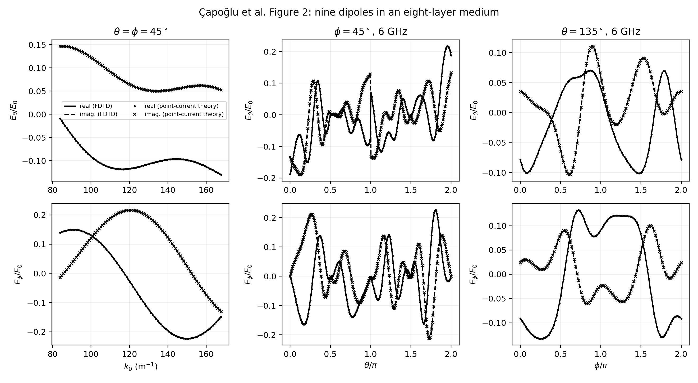
Fig. 97 Reproduction of the spectral, \(\theta\)-cut, and \(\phi\)-cut panels of Çapoğlu et al. Figure 2. Lines are the production FDTD Huygens-surface output and symbols are the direct point-current result.

The largest RMS difference of any real or imaginary curve, divided by that curve’s analytical peak, is 0.477 percent; the paper reports a maximum RMS error below one percent. Across all complex vector samples, the retained maximum and RMS errors normalised to the analytical vector peak are 0.378 and 0.271 percent, respectively.

Note

The numerator sign printed in Eq. (38) of [CAP2012] is opposite to the interface-reflection convention implied by Eqs. (18)–(30). gprMax uses the latter convention because it also recovers the required homogeneous- medium limit. The three-layer closed-form regression test records this choice explicitly.

Interfacial electric-dipole patterns

The interfacial-dipole validation compares the production transform with the asymptotic closed-form power patterns of Engheta, Papas, and Elachi [ENG1982]. Infinitesimal vertical and horizontal electric dipoles lie at an interface whose lower-to-upper refractive-index ratio is \(n=2\) or \(n=4\). For example, the normalised angular dependence of the vertical dipole in the upper half-space is proportional to

\[P_v(\theta)= \frac{n^4\sin^2\theta\cos^2\theta} {\left(n^2\cos\theta+ \sqrt{n^2-\sin^2\theta}\right)^2}, \qquad 0\leq\theta<\frac{\pi}{2}.\]

The independent reference implements the corresponding propagating and lateral-wave expressions in the lower half-space, and both principal-plane expressions for a horizontal dipole. The FDTD radial power is formed as

\[P_r(\theta,\phi)\ \propto \frac{|E_\theta|^2+|E_\phi|^2}{\eta_o(\theta)},\]

using the impedance of the observation half-space. Exact interface and critical-angle samples are excluded from error statistics because the asymptotic expressions are singular or change branch there.

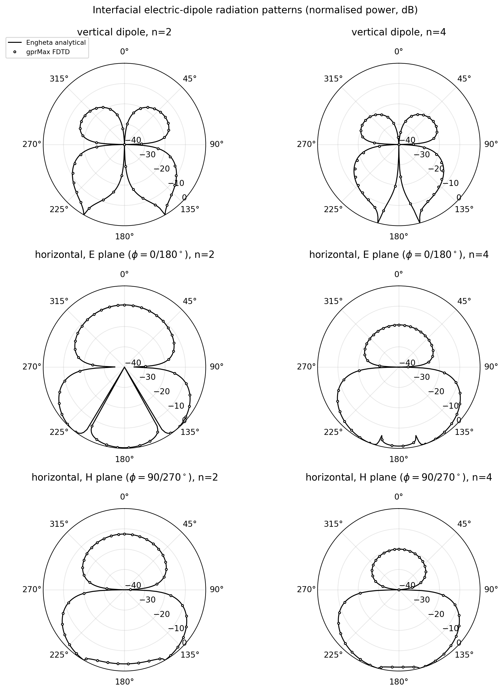
Fig. 98 Complete normalised-power cuts for vertical and horizontal interfacial dipoles. Lines are the Engheta analytical expressions and symbols are production gprMax results.

Across the six retained curves, the worst RMS normalised-power difference is 0.363 percent and the worst pointwise difference is 1.059 percent. The latter occurs for the vertical \(n=2\) case near a rapidly varying angular feature.

Finite-height dipole above a half-space

The Smith dipole-height validation places a horizontal electric dipole in air above a lossless \(\epsilon_r=9\) half-space. It evaluates the E- and H-plane patterns at 2 GHz for \(h/\lambda_0=0.1\), 0.2, and 0.35 against Smith’s asymptotic plane-wave-spectrum solution [SMI1984]. The finite height supplies the usual incident/reflected phase in the upper medium. In the lower-medium lateral-wave sector, its power multiplier is

\[A_h(\theta)=\exp\left[-2k_0h \sqrt{n^2\sin^2\theta-1}\right].\]

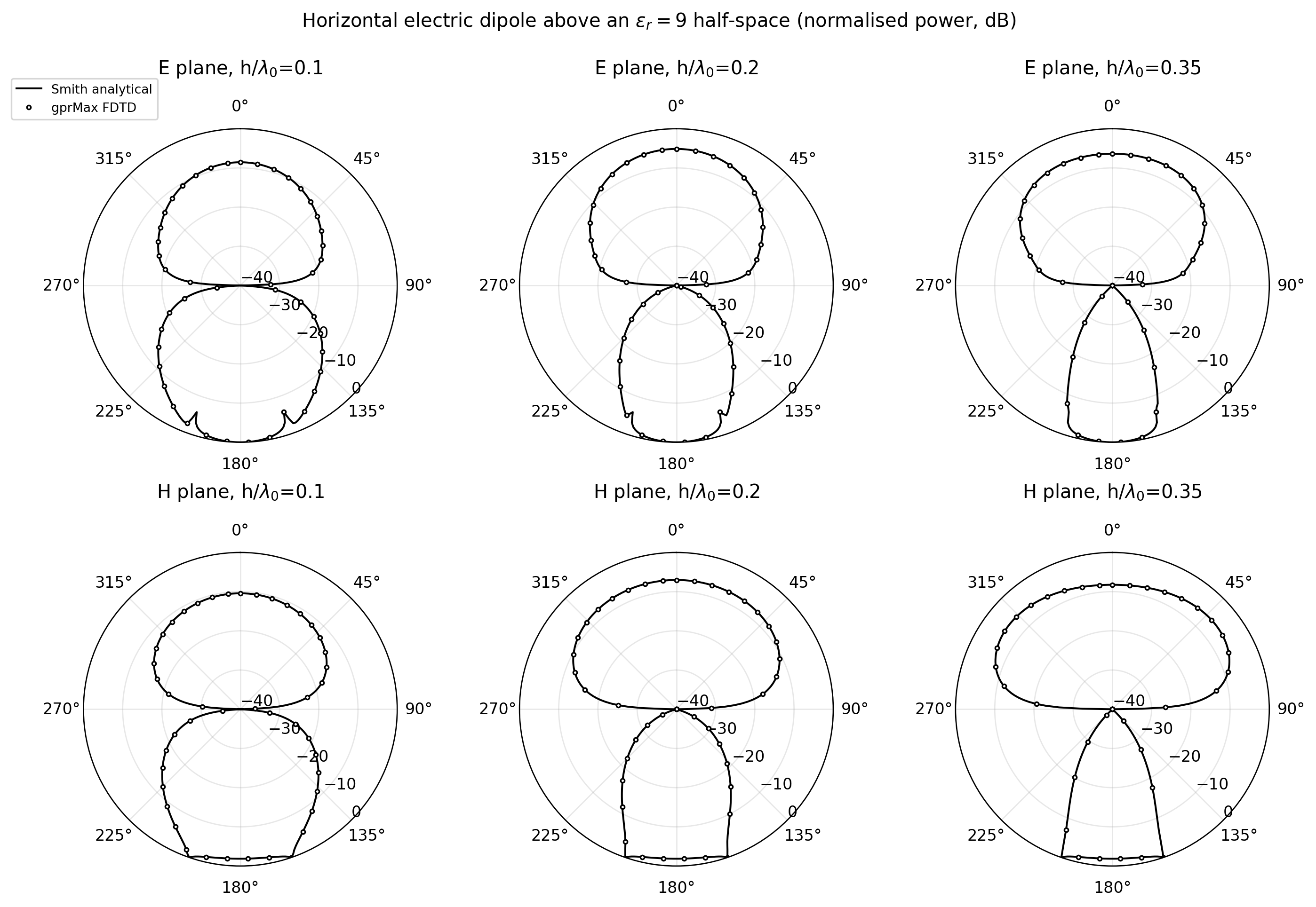
Fig. 99 Full E- and H-plane normalised-power patterns for the three source heights. Lines are Smith’s analytical result and symbols are gprMax.

The largest RMS normalised-power difference across all heights and cuts is 0.271 percent; the largest pointwise difference is 0.755 percent. These cases verify that the implementation retains the absolute source height and its direction-dependent phase or evanescent decay rather than treating every source as if it lay on the interface.

Finite-radius GPR antenna energy-pattern verification

This final layered-medium study is deliberately classified as a verification, not an independent analytical validation. The GSSI-like antenna driver reproduces the lossless \(\epsilon_r=5\) half-space configuration of Warren and Giannopoulos [WAR2017]. It samples the 1.5 GHz GSSI-like toolbox model at 25 radii from 0.10 to 0.58 m. At each radius the pulse-energy pattern is

\[\Psi_E(r,\theta)=\Delta t\sum_n |E_\theta(r,\theta,n)|^2,\]

with an analogous \(H_\theta\) measure for the H-plane. Every finite-radius curve is normalised by its own angular maximum. An asymptotic reference is calculated independently from those receiver circles using the closed layered NTFF surface,

\[\Psi_\infty(\theta)\ \propto \int_{0.1\,\mathrm{GHz}}^{4.0\,\mathrm{GHz}} |F_E(\theta,f)|^2\,\mathrm df.\]

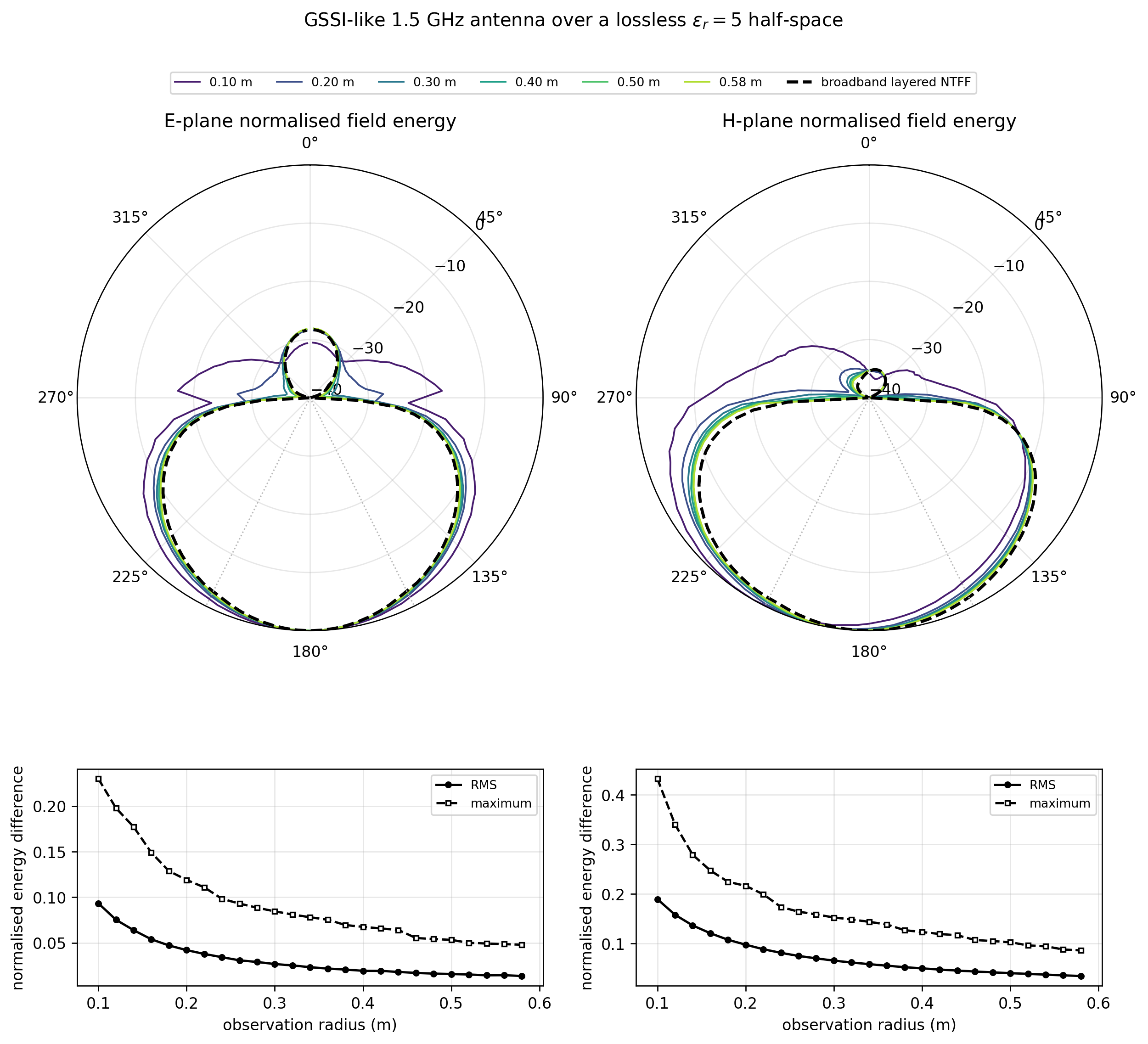
Fig. 100 Selected finite-radius energy patterns, the broadband layered-NTFF asymptote, and the pattern-shape difference as a function of radius. Zero degrees is directed into air and 180 degrees into the ground.

The reproduced curves show the convergence with increasing distance reported in the paper. The E-plane RMS difference from the broadband NTFF pattern falls from 9.34 percent at 0.10 m to 1.38 percent at 0.58 m; the H-plane difference falls from 18.94 to 3.44 percent. A Parseval check shows that the 0.1–4.0 GHz NTFF band contains 99.71 percent of aggregate E-plane record energy and 99.90 percent of H-plane energy.

The retained reproduction uses a 2 mm mesh, whereas the paper used 1 mm. The coarser mesh keeps the complete 0.58 m observation circle within one 24 GB GPU. No digitised published curve is used as an oracle: this calculation verifies the published convergence behaviour and agreement with the new asymptotic transform, rather than claiming pointwise agreement with the 2017 figure. The case note and retained metrics record the complete distinction.

Rational lumped networks in a parallel-plate guide

The rational-network validation driver uses the finite-width parallel-plate guide introduced by Pereda et al. [PER1999]. Its width is \(a=15\) mm, its plate separation is \(b=2\) mm, and the 1 mm Yee mesh gives 15 effective parallel paths, each containing two series electric edges. For a one-edge network impedance \(Z(\omega)\), the exact TEM quantities are therefore

\[Z_\mathrm{guide}=\eta_0\frac{b}{a},\qquad Z_\mathrm{sheet}=\frac{2Z}{15},\qquad \Gamma=-\frac{Z_\mathrm{guide}} {2Z_\mathrm{sheet}+Z_\mathrm{guide}}.\]

The FDTD result is obtained from an empty-guide incident run and a loaded-guide run. The first reflected pulse is isolated, transformed using the engineering Fourier convention, and de-embedded to the sheet with the axial Yee numerical wavenumber. Separate resistor, capacitor, and inductor sheets exercise the direct \(G\), direct \(sC\), and zero-pole terms. The two literature cases exercise a real pole for a series RC network and a conjugate pole pair for a series RLC network.

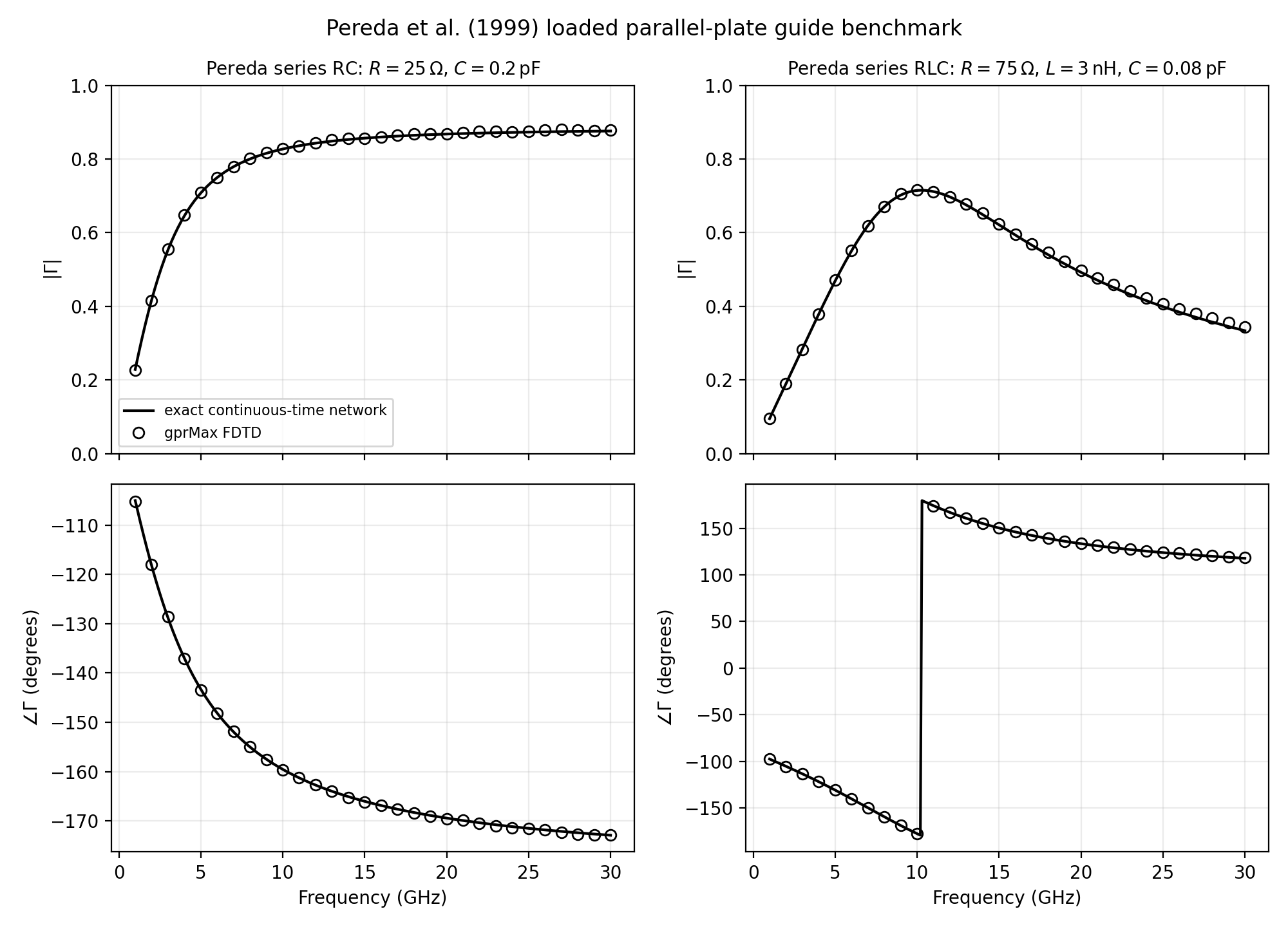
Fig. 101 Production gprMax FDTD reflection (symbols) compared with the exact continuous-time network result (lines) for the two examples of [PER1999].

From 1–30 GHz, the series-RC comparison has magnitude and phase RMS errors of 0.0027 and 0.15 degrees; the series-RLC errors are 0.0057 and 0.37 degrees. The RC capacitance printed in [PER1999] is 0.02 pF, but both magnitude and phase curves published in that paper correspond to 0.2 pF; the latter value is used for the reproduced curve above.

The arbitrary one-port coupling follows the lumped-network FDTD formulations of [PER1999] and [CHE2007]. gprMax does not retain their classic PLRC time placement unchanged. Each partial-fraction term is advanced using the exponential recursive-convolution approach of Giannakis and Giannopoulos [GIA2014], evaluated directly at \(n+1/2\) for a linearly varying terminal voltage. This avoids estimating the half-step network current by averaging adjacent integer-time pole currents.

Hertzian-dipole pattern, directivity, and near field

The Hertzian-dipole validation driver compares both KSIR and equivalent-current far fields with the analytical \(\sin\theta\) field pattern and \(D_\mathrm{max}=1.5\) directivity. It also compares one directly sampled and one KSIR-predicted time-domain near-field component with the complete analytical field.

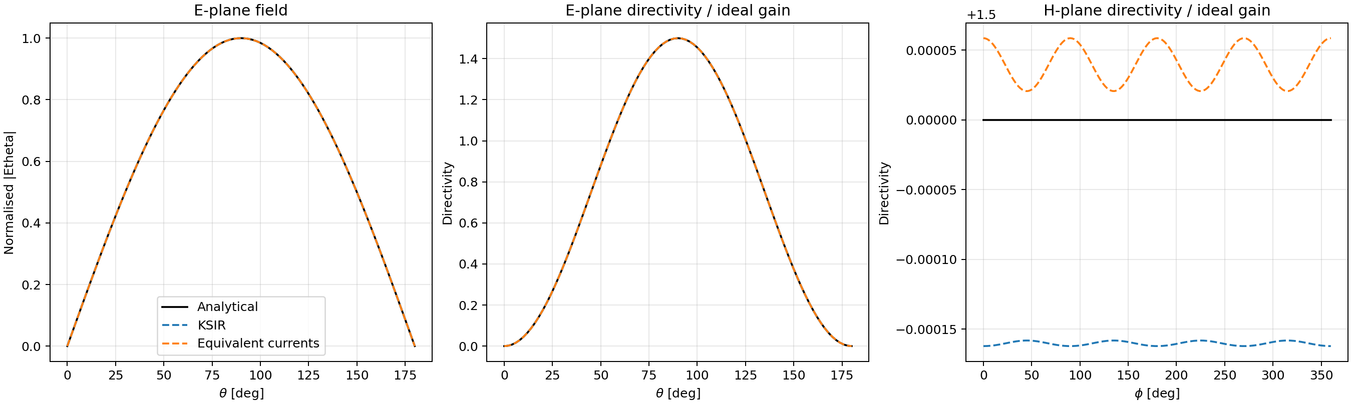
Fig. 102 Far-field pattern and directivity from both transformations compared with the Hertzian-dipole closed form.

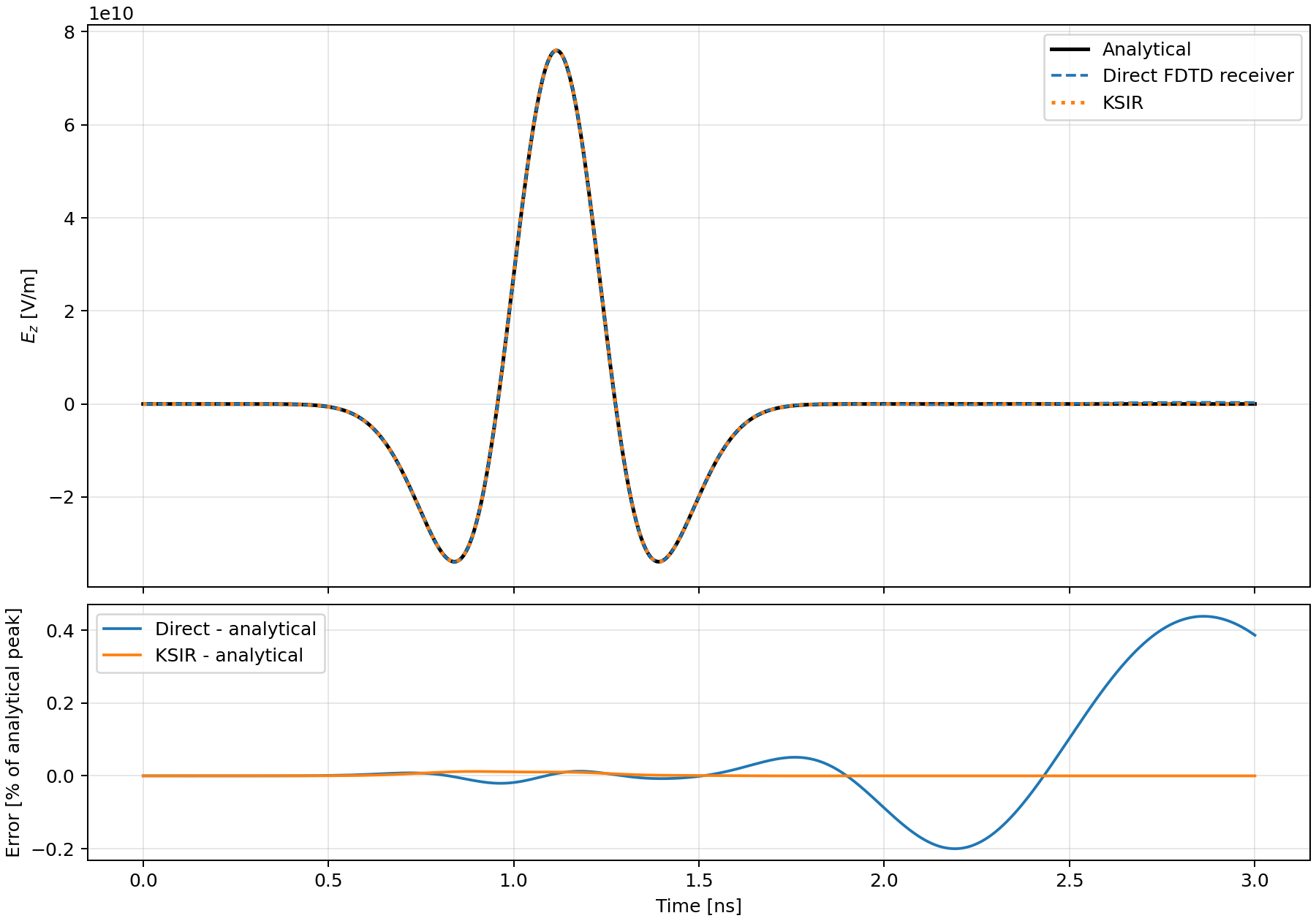
Fig. 103 Direct FDTD and KSIR time-domain near fields compared with the analytical component at the same physical position.

The retained result has directivity-pattern RMS errors below \(10^{-4}\) for KSIR and \(2.5\times10^{-5}\) for the equivalent-current method. The significant-signal relative L2 errors of the direct and KSIR near fields are \(3.4\times10^{-4}\) and \(1.7\times10^{-4}\), respectively.

Sphere radar cross section

The sphere studies illuminate a staircased sphere with a broadband discrete plane wave and calculate monostatic RCS using the production NTFF path. The reference values are evaluated independently from converged Mie series at the actual requested frequencies.

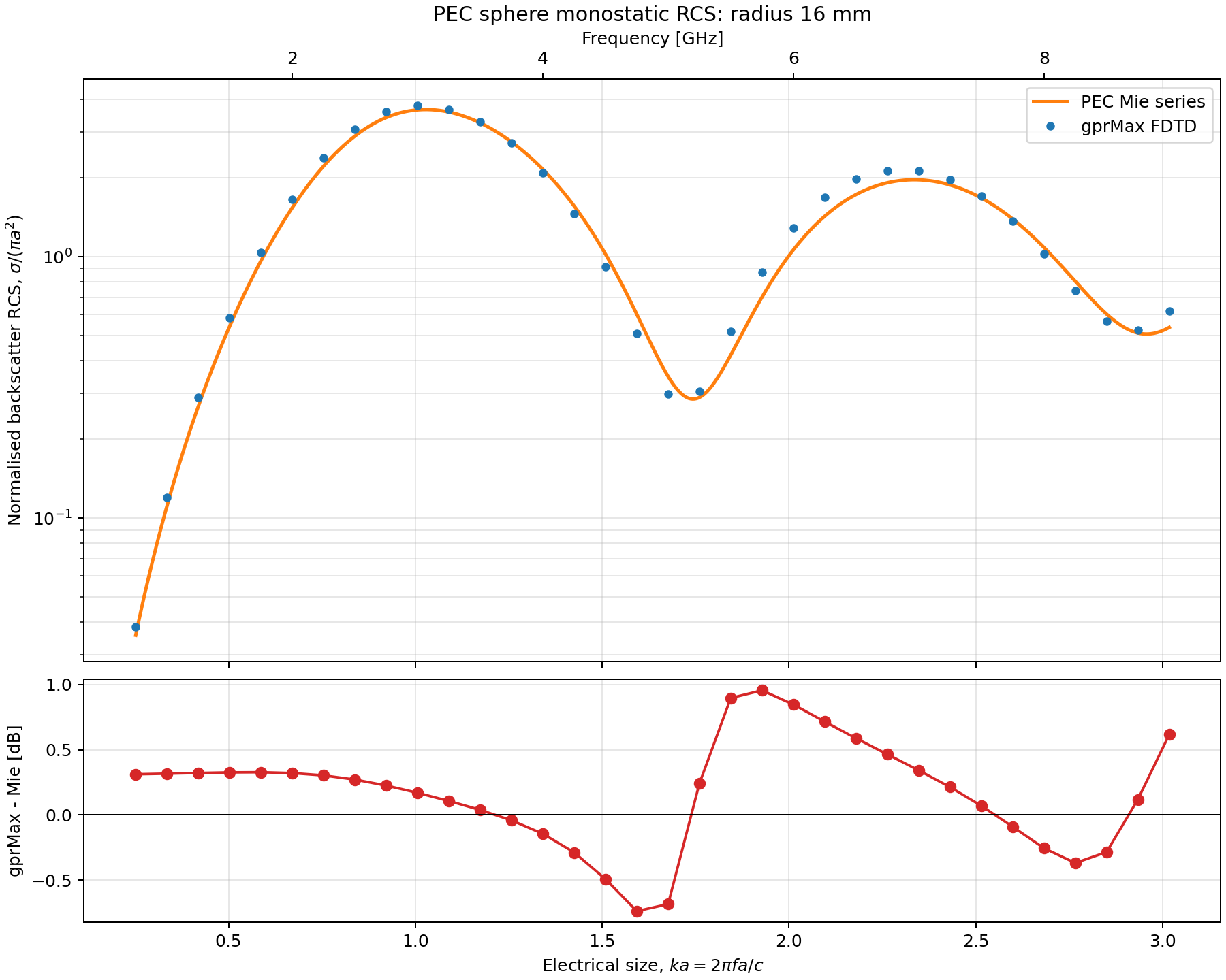
Fig. 104 Broadband PEC-sphere backscatter compared with the PEC Mie series.

The PEC-sphere driver covers \(0.25<ka<3.02\), including the first resonances and nulls. With a 0.5 mm grid and 16 mm radius, the retained result has 0.44 dB RMS error and 0.95 dB maximum error across 34 independent frequency samples.

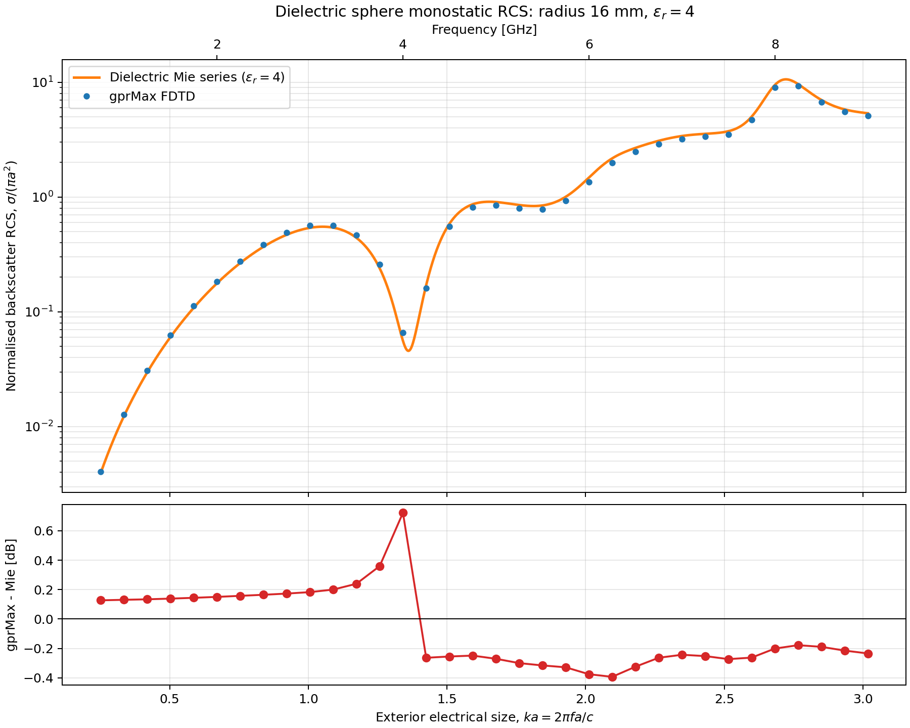
Fig. 105 Backscatter from a lossless \(\epsilon_r=4\) sphere compared with the homogeneous dielectric-sphere Mie series.

The dielectric-sphere driver uses the same exterior geometry and frequency range. Its retained result has 0.27 dB RMS error and 0.72 dB maximum error. This case additionally exercises dielectric geometry averaging and the shorter wavelength inside the sphere.

Dispersive spheres and interface averaging

Hartley’s effective-permittivity treatment extends the ordinary arithmetic electric-edge average to Debye media [HAR2020]. For the engineering Fourier convention used by gprMax, constituent material \(m\) has

\[\epsilon_{r,m}(\omega) = \epsilon_{\infty,m} + \sum_p \frac{\Delta\epsilon_{m,p}} {1 + j\omega\tau_{m,p}} + \frac{\sigma_m}{j\omega\epsilon_0}.\]

If the surrounding cells occupy fractions \(w_m\) of the contour-path area, with \(\sum_m w_m=1\), the effective edge response is

\[\epsilon_{r,\mathrm{eff}}(\omega) = \sum_m w_m\epsilon_{r,m}(\omega).\]

Consequently,

\[\begin{split}\begin{aligned} \epsilon_{\infty,\mathrm{eff}} &= \sum_m w_m\epsilon_{\infty,m}, \\ \sigma_{\mathrm{eff}} &= \sum_m w_m\sigma_m, \\ \Delta\epsilon_{\mathrm{eff},m,p} &= w_m\Delta\epsilon_{m,p}, \\ \tau_{\mathrm{eff},m,p} &= \tau_{m,p}. \end{aligned}\end{split}\]

The four cells surrounding a standard electric Yee edge each contribute \(w_m=1/4\). Repeated relaxation times are combined exactly; distinct times remain distinct poles. Thus two different single-pole Debye materials generally produce a two-pole interface material. This construction follows Chapter 4 of Hartley’s thesis [HAR2020].

The implementation extends the same arithmetic response to Lorentz and Drude media through the inclusive susceptibility used by gprMax [GIA2014]. If \(W_{m,p}\) and \(Q_{m,p}\) are the residue and location of a Debye, Lorentz, or Drude term, the interface retains \(Q_{m,p}\) and replaces \(W_{m,p}\) by \(w_m W_{m,p}\). Identical locations are merged exactly. This gives the frequency-by-frequency arithmetic constitutive response without fitting. It may, however, increase the model-wide pole count, so dispersive averaging is an opt-in feature.

Reducing this exact union is a separate, band-limited material-fitting problem. The validation package includes constrained fitting experiments, building on the type of hybrid optimisation used for Debye fitting in [KEL2007], but the production solver never replaces the exact interface response automatically.

The Debye-sphere averaging driver reproduces the three curved-interface experiments from Section 4.4 of the thesis. A \(200^3\) grid contains a sphere of radius 60 cells made from one of three two-pole Puerto Rico clay/loam models. A 300 MHz discrete plane wave excites the model, and production equivalent-current NTFF output is compared from 25 to 525 MHz with an independent homogeneous dispersive-sphere Mie series.

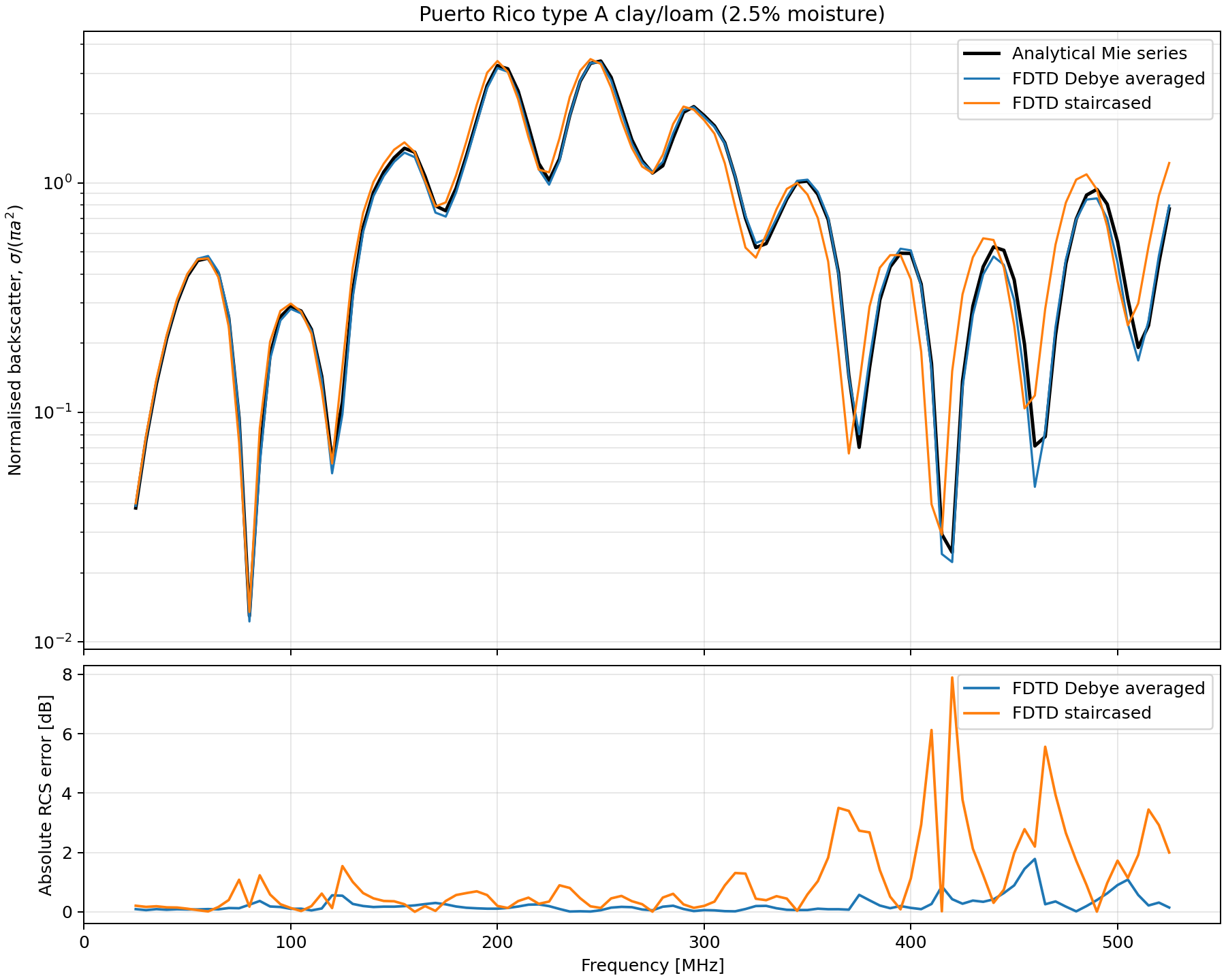
Fig. 106 Type A clay/loam (2.5% moisture): analytical Mie backscatter compared with dispersive-averaged and non-averaged FDTD spheres.

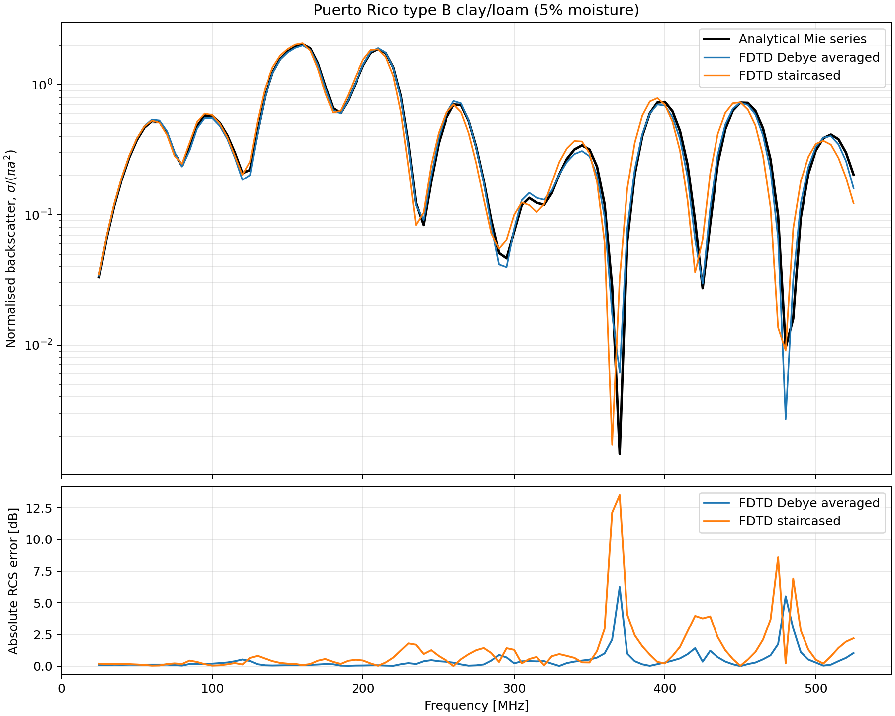
Fig. 107 Type B clay/loam (5% moisture). Debye averaging follows the resonant minima more closely than the staircased interface.

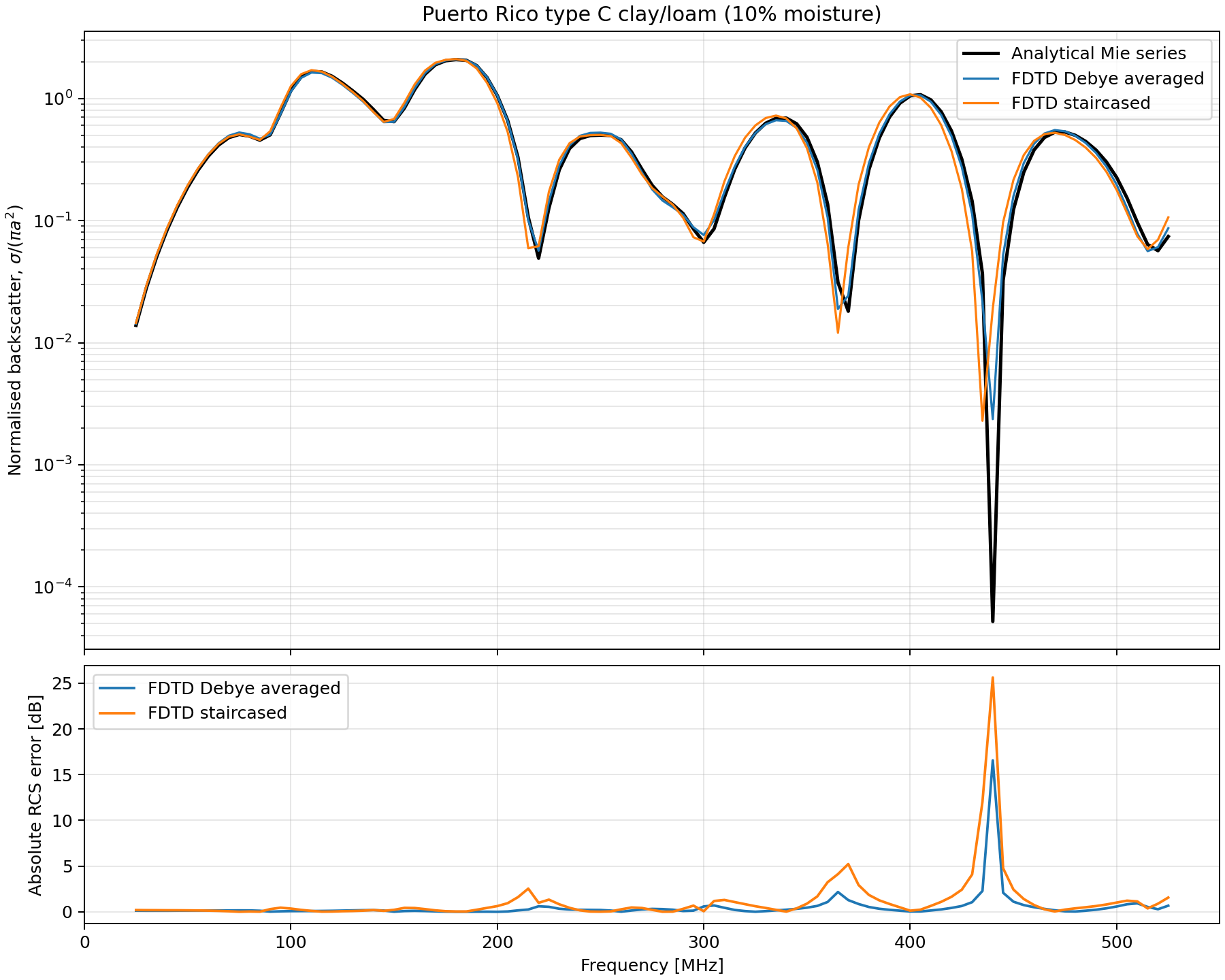
Fig. 108 Type C clay/loam (10% moisture). Errors in dB become very large at the exceptionally deep analytical null, so global relative L2 error is the more representative metric.

The retained 300 ns simulations give:

Table 31 Debye-sphere backscatter errors

Soil	Averaged RMS error	Staircased RMS error	Averaged relative L2	Staircased relative L2
A, 2.5%	0.371 dB	1.728 dB	3.39%	13.71%
B, 5%	1.011 dB	2.476 dB	3.58%	11.57%
C, 10%	1.734 dB	3.090 dB	3.14%	8.85%

The relative L2 error is reduced by factors of approximately 4.0, 3.2, and 2.8 for soils A, B, and C, respectively. Unlike the planar half-space test, these curved objects expose the geometric and accumulated phase errors that the interface average is intended to reduce.

Mixed dispersive layers and a core-shell sphere

The reusable validation modules in testing/validation/dispersive_averaging extend the comparison to mixed dispersion families. Planar stacks are evaluated with the normal-incidence multilayer recursion using the complex permittivity of every layer. All FDTD results are de-embedded to the geometrical first interface requested by the model; no fitted half-cell displacement is applied.

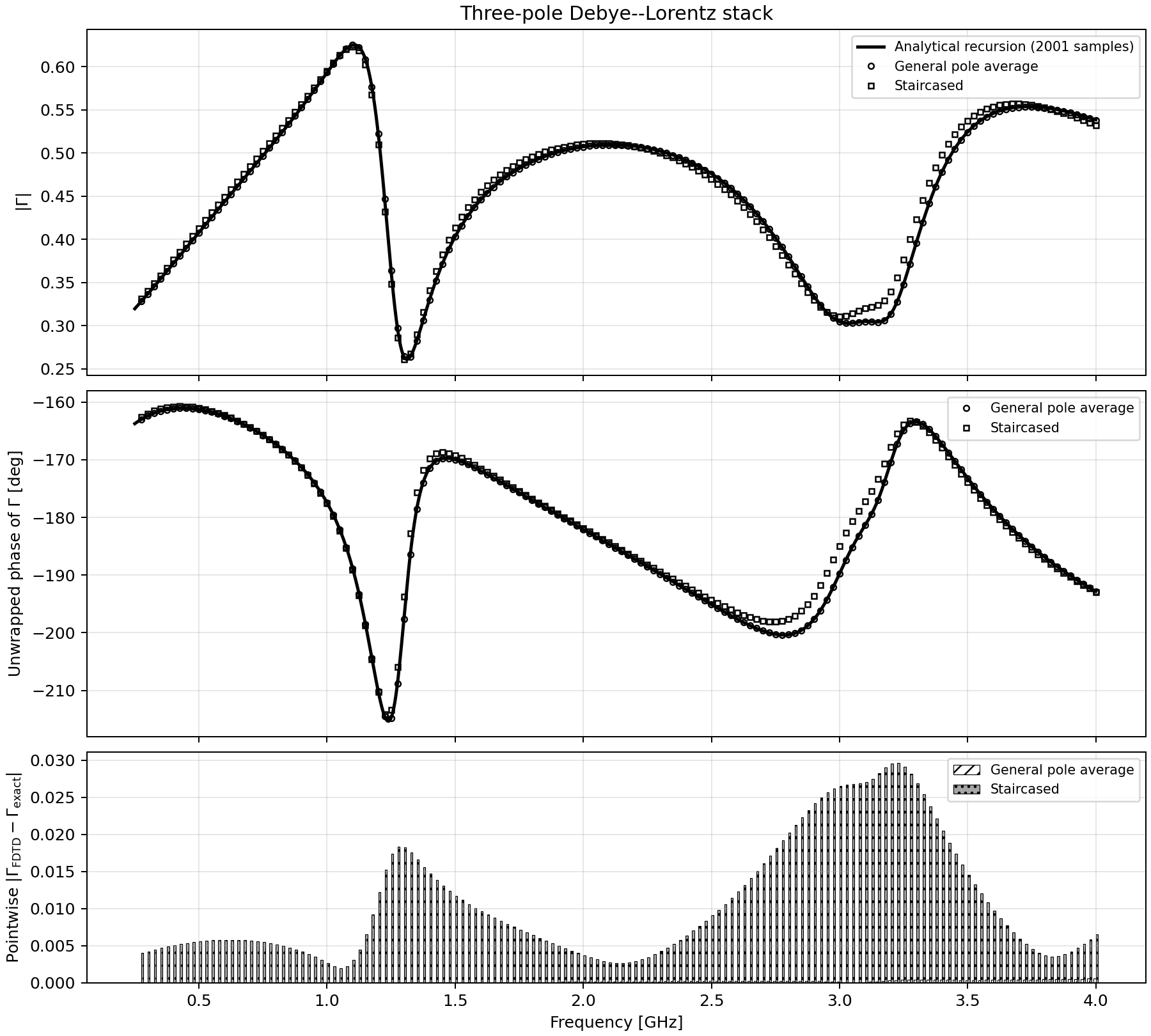
Fig. 109 A three-pole Debye layer and a two-pole Lorentz layer compared with the analytical multilayer reflection coefficient. Symbols are FDTD samples; the continuous black curve is evaluated independently.

Across the retained dielectric, Debye/dielectric, Debye/Lorentz, Lorentz/Drude, and multipole Debye/Lorentz stacks, exact interface averaging gives complex relative L2 errors between \(4.3\times10^{-4}\) and \(8.1\times10^{-4}\). The corresponding staircased errors are 1.85–3.70%. The multilayer validation driver also records magnitude and phase residuals at every FDTD frequency.

The curved mixed-material test is a 60 mm Debye core surrounded by a 100 mm outer-radius Lorentz shell. Its exact backscatter reference uses the Aden–Kerker coated-sphere series and the complex material response at every frequency.

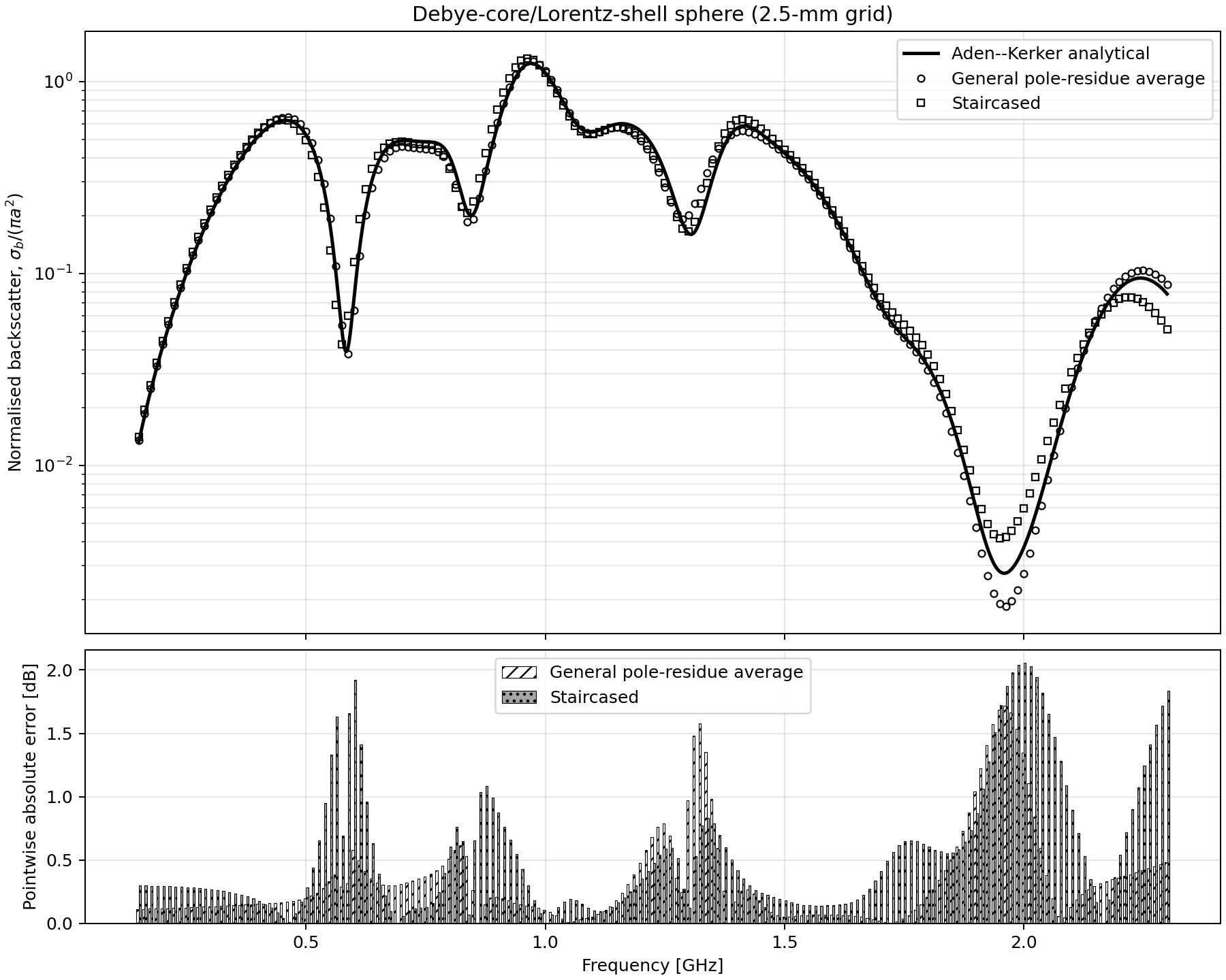
Fig. 110 Refined Debye-core/Lorentz-shell backscatter. The analytical curve is densely sampled; averaged and staircased FDTD results are shown as symbols with pointwise error bars below.

On the 2.5 mm grid, the exact pole-residue average reduces the complex relative L2 error from 8.77% to 6.01% and the RMS logarithmic error from 0.756 dB to 0.507 dB. Run the coated-sphere validation driver to regenerate the full comparison.

Tagged-cell SAR in a lossy half space

The SAR validation driver launches a normally incident unit-amplitude plane wave onto a homogeneous conductive half space whose declared interface uses dielectric averaging. It compares cell-centred SAR along the central propagation line with the Fresnel transmitted field and its analytical attenuation. The analytical field is integrated over the cell volume, as recommended for comparisons of FDTD SAR algorithms [LAA2010]. A secondary implementation-matched comparison averages the two tangential electric-field phasors on the bounding faces of the cell:

\[\begin{split}\begin{aligned} E(z) &= \frac{2\eta_2}{\eta_1+\eta_2}\exp(-\gamma_2 z),\\ E_c(z) &= \frac{E(z-\Delta x/2)+E(z+\Delta x/2)}{2},\\ \overline{\mathrm{SAR}}(z) &= \frac{1}{\Delta x} \int_{z-\Delta x/2}^{z+\Delta x/2} \frac{\sigma |E(u)|^2}{2\rho}\,\mathrm{d}u. \end{aligned}\end{split}\]

For the supplied 1 GHz, 2 mm-grid case, the production on-the-fly transform has a relative L2 error of 0.113% and a maximum pointwise relative error of 0.150% against the exact cell-volume average over 16 interior depth samples. The implementation-matched Yee-collocated errors are 0.072% and 0.093%.

One broadband run also evaluates 14 frequencies from 0.5 to 7 GHz. The cell-average L2 error rises smoothly from 0.040% at 0.5 GHz to 5.69% at 7 GHz, where the shortest wavelength has 10.7 cells. The corresponding maximum pointwise errors are 0.041% and 7.00%. This shows both the accuracy of the on-the-fly multi-frequency transform and the expected deterioration as the grid approaches its lambda/10 limit. The script enforces conservative 5% and 6% limits for its default 1 GHz test and writes plots plus JSON metrics.

This is the local-SAR analytical validation. The separate spatial-average validation driver compares the production 1 g/10 g algorithm with the independent Apache-2.0 STASIS implementation of IEC/IEEE 62704-1. For its heterogeneous two-density test, all voxel-status classifications agree. The maximum relative differences in spatial-average SAR are \(5.14\times10^{-8}\) for 1 g and \(9.90\times10^{-6}\) for 10 g; the residual is attributable to the two implementations’ independent cubic-root searches. The external reference repository is not bundled with gprMax and must be supplied to the driver.

The exhaustive comparison with the official uniform-grid SAR Star reports uses a \(281^3\) grid containing 1,498,184 tissue voxels. For both 1 g and 10 g there are zero tissue-status, background-status, and unambiguous orientation mismatches. For 1 g, the maximum relative mass, volume, and SAR differences are \(2.17\times10^{-7}\), \(1.95\times10^{-7}\), and \(7.55\times10^{-7}\). For 10 g they are \(2.00\times10^{-7}\), \(1.75\times10^{-7}\), and \(7.50\times10^{-7}\). With reusable averaging geometry and compiled OpenMP processing, the complete 1 g and 10 g cases took 20.9 s and 36.9 s, respectively, on the validation server. Before this optimisation the same production algorithm took 4,710 s and 3,555 s. These full-size comparisons remain manual release validations rather than routine CI tests.

Tagged-cell SAR in a lossy dielectric sphere

The lossy-sphere SAR driver supplies an independent three-dimensional check that includes a curved, staircased material boundary. A unit-amplitude plane wave illuminates a homogeneous conductive dielectric sphere. The exact Mie absorption cross-section is

\[C_{\mathrm{abs}} = \frac{2\pi}{k_0^2} \sum_{n=1}^{\infty}(2n+1) \left[\Re(a_n+b_n)-|a_n|^2-|b_n|^2\right],\]

where \(a_n\) and \(b_n\) are the homogeneous-sphere Mie coefficients [MIE1908]. For an incident peak electric-field phasor \(E_0\), the reference absorbed power is

\[P_{\mathrm{abs}}^{\mathrm{Mie}} = C_{\mathrm{abs}}\frac{|E_0|^2}{2\eta_0}.\]

The production gprMax result is evaluated independently by integrating the tagged-cell absorbed-power-density output, \(P_{\mathrm{abs}}^{\mathrm{FDTD}}=\sum_i p_{\mathrm{abs},i}\Delta V\). The same run requests an incident_flux-normalised radiometry output, for which the tag integral is the absorption cross-section directly. Thus the validation exercises both the density-dependent SAR route and the density-independent radiometric weighting route against one independent Mie quantity. For the supplied 18 mm-radius, \(\epsilon_r=4\), \(\sigma=0.3\) S/m sphere at 1 GHz, the relative absorbed-power errors decrease from 12.29% to 8.81% and 6.37% as the resolution increases from 12 to 18 and 24 cells per radius. Double-precision CUDA runs at 36 and 48 cells per radius reduce the error further to 4.27% and 3.29%, respectively. The monotonic convergence is consistent with curved-interface staircasing and ordinary FDTD discretisation, rather than agreement to numerical precision.

Two-dimensional SAR in lossy dielectric cylinders

The 2-D cylinder SAR validation driver compares production TMz and TEz SAR with the exact internal fields of a homogeneous, lossy, infinite circular cylinder. The general oblique-incidence cylindrical-wave solution was derived by Wait [WAI1955]; at normal incidence the two polarisations decouple and the cross-polarised field vanishes.

Gasmelseed [GAS2026] used a muscle cylinder to check a separate 2-D FDTD implementation before studying numerical-dispersion compensation in layered tissues. That paper presents a graphical TMz cylinder comparison but does not report numerical cylinder-error estimates. The error measures below are new gprMax validation results. No medium-scaling or dispersion-correction method from that paper is used: the test uses the declared physical material properties directly.

Exact cylindrical series

For the \(\exp(j\omega t)\) convention, define

\[\widetilde{\epsilon}_r = \epsilon_r + \frac{\sigma}{j\omega\epsilon_0}, \qquad m=\sqrt{\widetilde{\epsilon}_r}, \qquad \widetilde{\epsilon}=\epsilon_0\widetilde{\epsilon}_r, \qquad k_0=\frac{\omega}{c}, \qquad k_1=mk_0, \qquad x=k_0a,\]

where \(a\) is the cylinder radius. A unit-amplitude plane wave travelling in the positive x direction has the cylindrical expansion

\[\exp(-jk_0r\cos\phi) = \sum_{n=-\infty}^{\infty} (-j)^nJ_n(k_0r)\exp(jn\phi).\]

For TMz, the exact internal axial electric field is

\[E_z^{\mathrm{int}}(r,\phi) = E_0\sum_{n=-\infty}^{\infty} (-j)^n B_n^{\mathrm{TM}} J_n(k_1r)\exp(jn\phi),\]

with

\[B_n^{\mathrm{TM}} = \frac{ J_n(x)H_n^{(2)\prime}(x)-J_n'(x)H_n^{(2)}(x) }{ J_n(mx)H_n^{(2)\prime}(x) -mJ_n'(mx)H_n^{(2)}(x) }.\]

For TEz, \(H_z\) is the axial scalar field and \(E_z=0\):

\[H_z^{\mathrm{int}}(r,\phi) = H_0\sum_{n=-\infty}^{\infty} (-j)^n B_n^{\mathrm{TE}} J_n(k_1r)\exp(jn\phi),\]

\[B_n^{\mathrm{TE}} = \frac{ J_n(x)H_n^{(2)\prime}(x)-J_n'(x)H_n^{(2)}(x) }{ J_n(mx)H_n^{(2)\prime}(x) -m^{-1}J_n'(mx)H_n^{(2)}(x) }.\]

The transverse TE electric fields follow directly from Maxwell’s equations,

\[E_r = \frac{1}{j\omega\widetilde{\epsilon}r} \frac{\partial H_z}{\partial\phi}, \qquad E_\phi = -\frac{1}{j\omega\widetilde{\epsilon}} \frac{\partial H_z}{\partial r}.\]

The series is truncated after

\[N=\left\lceil X+4.05X^{1/3}+12\right\rceil, \qquad X=\max\left(|k_0a|,|k_1a|\right),\]

and is evaluated from \(n=-N\) to \(N\). The validator reconstructs the scattered coefficients and independently checks continuity of the scalar field and its appropriately weighted normal derivative at \(r=a\). Across the retained cases, the largest relative boundary residual is \(6.1\times10^{-16}\).

SAR comparison and error measures

The exact complex fields are evaluated at the actual gprMax Yee-edge locations and collocated to the cell centre using the same TM/TE rules as the production implementation described in Absorbed power density and specific absorption rate. Complex fields are averaged before their magnitude is taken. With peak phasors, the analytical local SAR is [IEEE62704-3]

\[\mathrm{SAR}_{\mathrm{TM}} = \frac{\sigma}{2\rho}|E_z|^2, \qquad \mathrm{SAR}_{\mathrm{TE}} = \frac{\sigma}{2\rho} \left(|E_r|^2+|E_\phi|^2\right).\]

The continuous absorbed power per unit invariant length is evaluated as

\[P'_{\mathrm{abs}} = \frac{\sigma}{2}\int_0^a\int_0^{2\pi} |\mathbf{E}(r,\phi)|^2r\,\mathrm{d}\phi\,\mathrm{d}r.\]

The radiometry output is checked independently as an absorption cross-section per unit invariant length,

\[C'_{\mathrm{abs}}=\frac{P'_{\mathrm{abs}}}{S_{\mathrm{inc}}}.\]

Its relative error is identical to \(\epsilon_P\), as required. For the reported muscle case it is 0.949% for TMz and 0.232% for TEz; the latter is an exact-series extension rather than a value reported by Gasmelseed.

For TMz, angular orthogonality gives

\[P'_{\mathrm{abs,TM}} = \pi\sigma|E_0|^2 \sum_{n=-\infty}^{\infty}|B_n^{\mathrm{TM}}|^2 \int_0^a|J_n(k_1r)|^2r\,\mathrm{d}r.\]

The radial integrals for both modes are evaluated using 600-point Gauss–Legendre quadrature. Increasing the quadrature order from 300 to 600 changes the muscle-cylinder reference by approximately \(1.2\times10^{-13}\) relative.

For the selected cell set \(\mathcal{I}\), the reported local and integrated errors are

\[\begin{split}\begin{aligned} \epsilon_{L_2} &= \frac{\left\|\mathrm{SAR}_{\mathrm{FDTD}} -\mathrm{SAR}_{\mathrm{Mie}}\right\|_2} {\left\|\mathrm{SAR}_{\mathrm{Mie}}\right\|_2},\\ \epsilon_{\max} &= \max_{i\in\mathcal{I}} \frac{\left|\mathrm{SAR}_{i,\mathrm{FDTD}} -\mathrm{SAR}_{i,\mathrm{Mie}}\right|} {\mathrm{SAR}_{i,\mathrm{Mie}}},\\ \epsilon_P &= \frac{\left|P'_{\mathrm{FDTD}}-P'_{\mathrm{Mie}}\right|} {P'_{\mathrm{Mie}}}. \end{aligned}\end{split}\]

Cells below 5% of the analytical peak SAR are excluded from the local relative metrics. The primary interior metric additionally excludes a two-cell band at the cylinder boundary. This separates field-update accuracy from the inevitable geometrical difference between an exact circular interface and a voxelised, dielectrically averaged Yee interface. All-cell results are still written to the JSON report.

Numerical cases and results

The cylinders have radius 60 mm and are illuminated at 5.5 GHz by a grid-axis-aligned discrete plane wave travelling along the positive x direction, normal to the cylinder’s invariant z axis. A completed 3.5 GHz Ricker waveform provides a strong 5.5 GHz spectral component without the position-dependent finite-record bias of a truncated continuous sine. The model uses 0.4 mm cells, an 8 ns time window, 12-cell exterior PMLs, and dielectric averaging on the circular interface. The target incident electric field is 1 V/m. The electrical properties are the physical skin, fat, and muscle values reported by Gasmelseed [GAS2026]; the two former materials are applied to cylinders here as additional tests. Representative tissue densities scale absolute SAR equally in both solutions and do not affect the relative electromagnetic errors.

Table 32 CUDA double-precision cylinder validation at 0.4 mm resolution

Material	\(\epsilon_r\)	\(\sigma\) (S/m)	Mode	Interior \(\epsilon_{L_2}\)	Interior \(\epsilon_{\max}\)	\(\epsilon_P\)
Fat	4.983	0.274	TMz	0.32%	1.33%	0.19%
Fat	4.983	0.274	TEz	0.72%	11.52%	0.062%
Skin	35.36	3.463	TMz	2.80%	8.88%	0.73%
Skin	35.36	3.463	TEz	2.56%	14.98%	0.038%
Muscle	48.9	4.61	TMz	3.46%	11.51%	0.95%
Muscle	48.9	4.61	TEz	3.02%	15.40%	0.23%

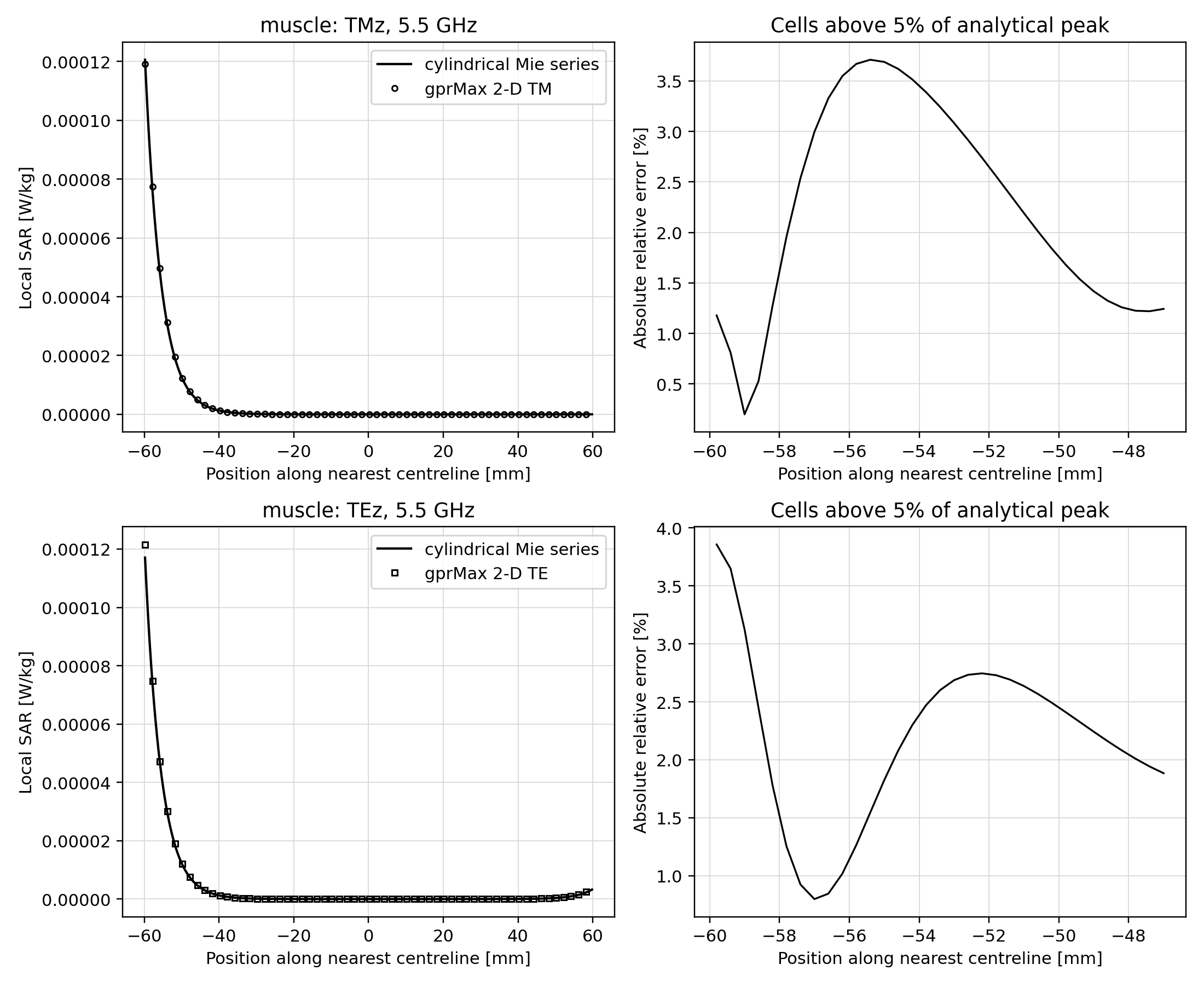
Fig. 111 Centreline local SAR for the muscle cylinder. Solid curves are the exact cylindrical series; symbols are gprMax samples.

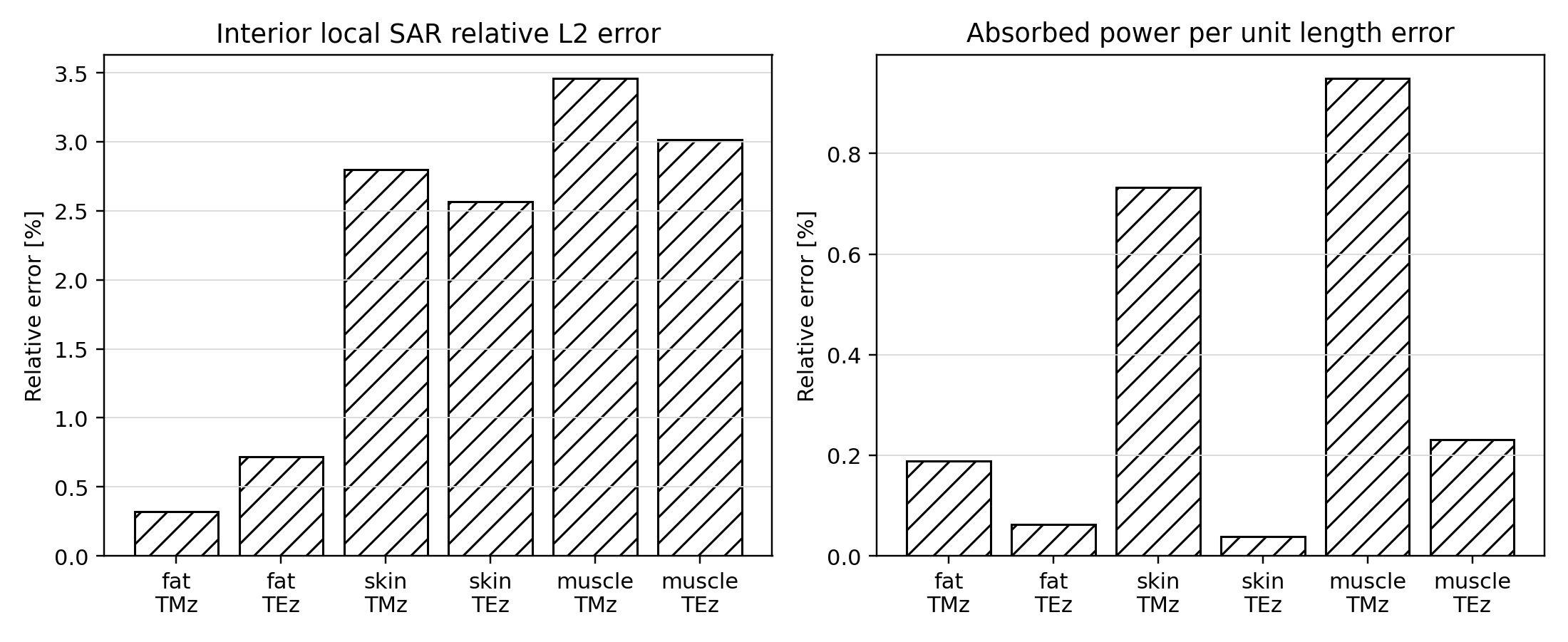
Fig. 112 Interior local-SAR and integrated absorbed-power errors for the three materials and both polarisations.

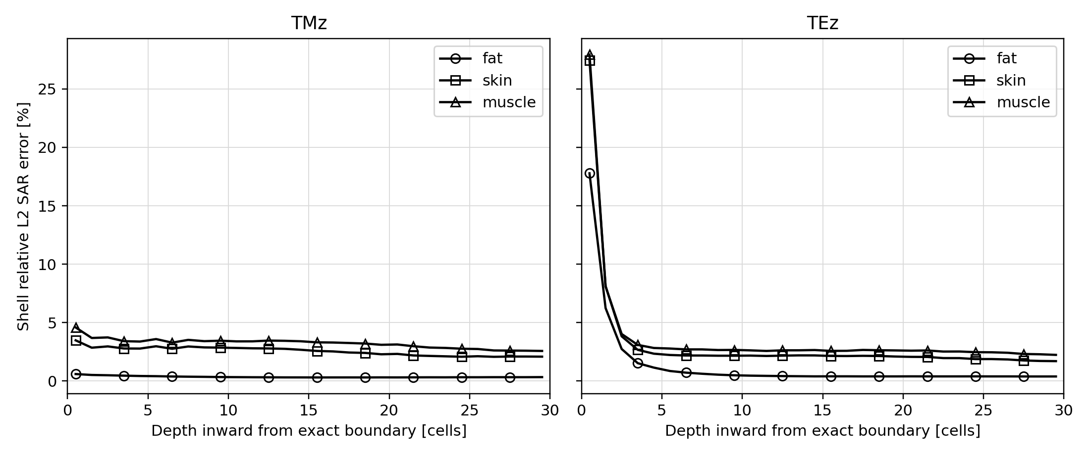
Fig. 113 Shell-wise error versus distance from the exact interface. TEz is more sensitive to the representation of the discontinuous tangential electric field, but the excess error is strongly concentrated in the first two boundary-cell layers.

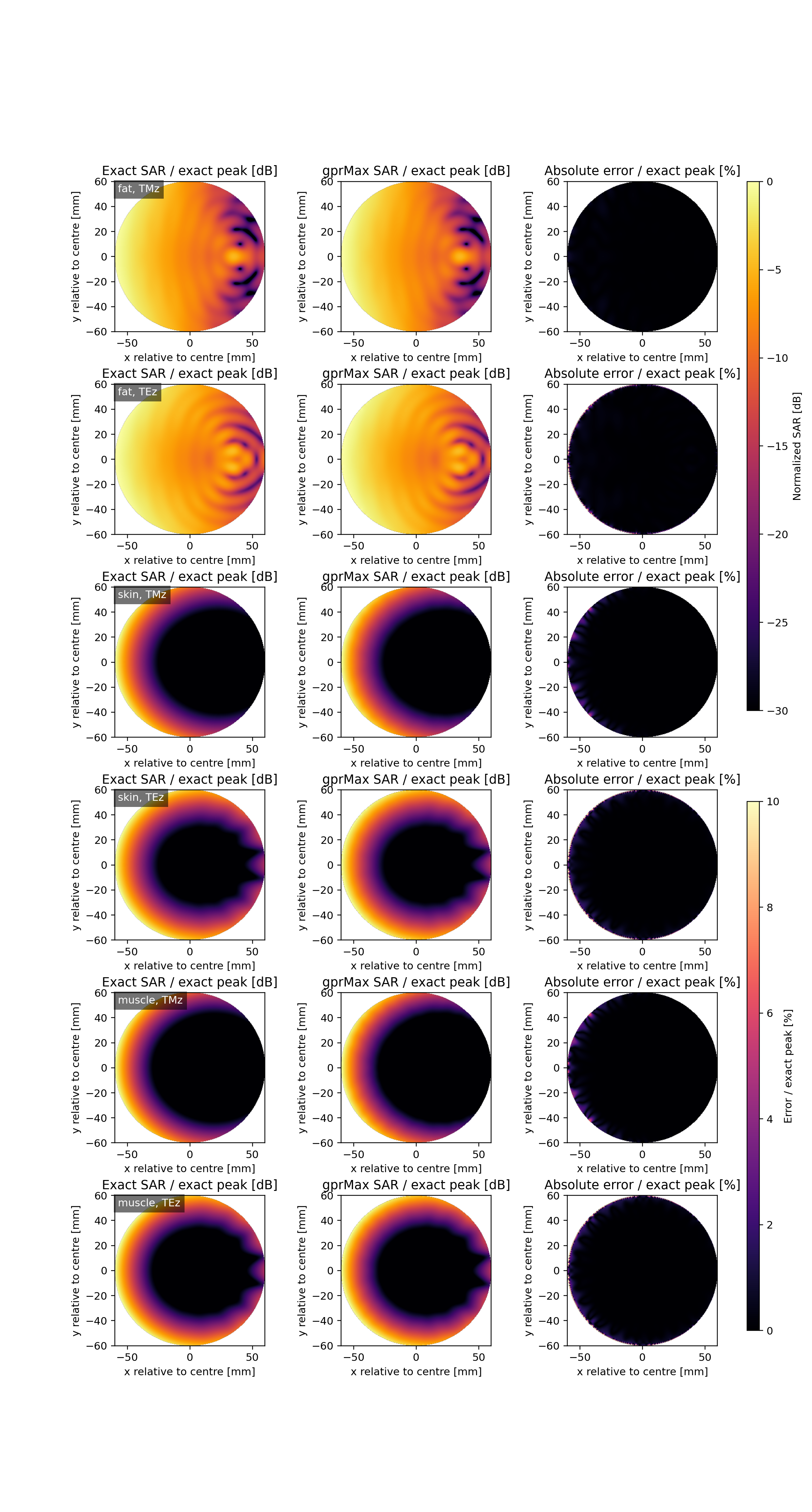
The full two-dimensional field maps show the exact and gprMax SAR distributions and error normalised by the exact peak. Halving the muscle TMz cell size from 0.4 to 0.2 mm reduces the interior \(\epsilon_{L_2}\) from 3.46% to 0.72% and \(\epsilon_P\) from 0.95% to 0.22%, demonstrating mesh convergence. CPU and CUDA double-precision muscle results agree to \(5.9\times10^{-13}\) relative L2 for TMz and \(1.7\times10^{-12}\) for TEz.

The retained material cases can be regenerated from the repository root, for example:

python -m testing.validation.validate_sar_2d_cylinder \
    --backend cuda --precision double --material muscle --modes TM TE

Replace muscle by fat or skin to reproduce the other rows. The driver writes the complete parameters, checks, and unrounded errors to its JSON report rather than relying on values read from a plotted curve.

Power-normalisation consistency

The power-normalisation driver exercises an actual voltage source and its automatic port through the complete solver and output path. Requesting 4 W rather than 1 W incident power multiplies every SAR value by four exactly. Normalising the same fields to accepted rather than incident power agrees with the independently evaluated port-power ratio to \(8.9\times10^{-16}\) relative. This test establishes implementation consistency; unlike the half-space and sphere cases, it is not an independent electromagnetic reference solution.

Running the validation suite

Run the studies from the repository root, for example:

python -m testing.validation.validate_plane_wave_dispersive_halfspace --gpu 0
python -m testing.validation.validate_plane_wave_realistic_materials --gpu 0
python -m testing.validation.validate_hertzian_dipole --gpu 0
python -m testing.validation.validate_rational_network_literature
python -m testing.validation.validate_pec_sphere_rcs --gpu 0
python -m testing.validation.validate_dielectric_sphere_rcs --gpu 0
python -m testing.validation.validate_debye_sphere_averaging --gpu 0
python -m testing.validation.validate_sar_lossy_halfspace
python -m testing.validation.validate_sar_lossy_sphere
python -m testing.validation.validate_sar_2d_cylinder \
    --backend cuda --precision double --material muscle --modes TM TE
python -m testing.validation.validate_sar_power_normalisation
python testing/validation/validate_sar_spatial_averaging.py \
    --reference /path/to/IEC-IEEE-62704-1-spatial-average-SAR
python -m testing.validation.validate_sar_star \
    /path/to/62704-1_supplemental_files.zip
python -m testing.validation.dispersive_averaging.validate_multilayer_fdtd
python -m testing.validation.dispersive_averaging.validate_core_shell_fdtd --gpu 0
python -m gprMax \
    testing/validation/rectangular_waveguide_partial_cutoff/rectangular_waveguide_partial_cutoff.in \
    --hide-progress-bars
python testing/validation/rectangular_waveguide_partial_cutoff/plot_partial_cutoff.py

Omit --gpu for CPU execution. The full-resolution plane-wave and sphere cases are long-running and are not part of the default pytest selection. See the validation README for the output layout, cache policy, and acceptance criteria.

Related half-wave dipole example

The wire-dipole antenna example demonstrates the simulated reflection coefficient, input impedance, directivity, and gain of a finite half-wave dipole. Its resonant frequency and impedance can be compared with classical thin-wire predictions, while the more detailed MoM comparison is documented in the numerical-comparison section.