Advanced features

This section provides example models of some of the more advanced features of gprMax. Each example comes with an input file which you can download and run.

Eigenmode ports

The nine numbered examples under examples/features/eigenmode_ports progress from straight and curved guides to a closed-surface horn, a complete modal matrix study, a phase-steered array, a guide crossing cutoff, and physically aligned degenerate circular TE11 modes. Examples 8 and 9 demonstrate the experimental automatic tracker on an automatically detected TE11 pair and a true crossing of two polarized branches in an anisotropic waveguide. Automatic tracking requires further testing and should be used at the user’s discretion; legacy tracking remains the default. Eigenmode ports and S-parameter analysis provides a step-by-step tutorial for users who primarily want S-parameters and far fields.

Always inspect the solved mode before committing to a long FDTD run:

python examples/features/eigenmode_ports/example_1_straight_waveguide/straight_waveguide.py --geometry-only

Geometry-only mode builds the material grid and solves the mode without time stepping. It automatically writes the modal-field plot. Check its requested polarisation, symmetry, mode order, confinement, and field behaviour at material, PEC, or PMC boundaries.

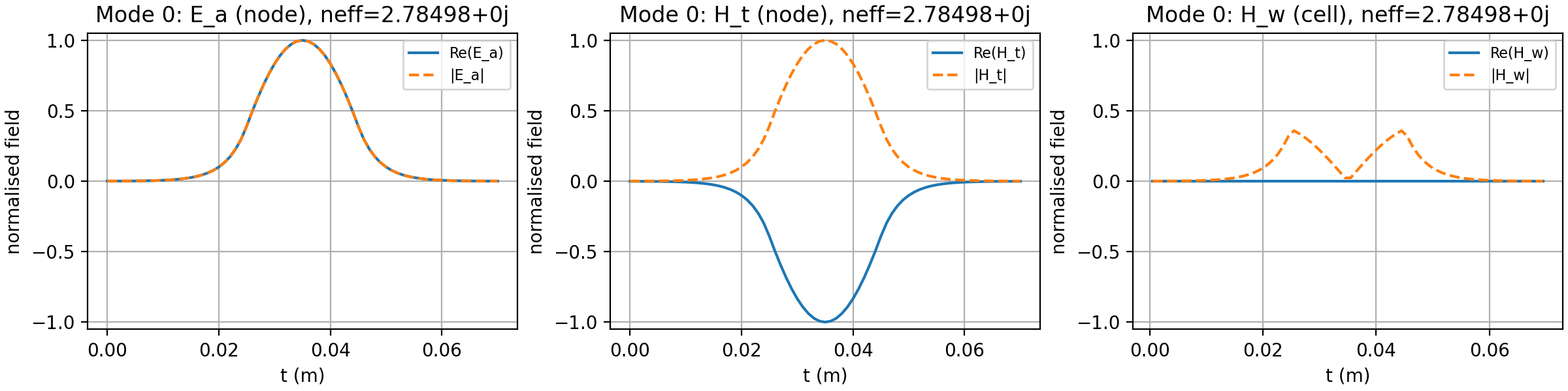
Fig. 32 Yee-staggered active field components of the fundamental 2D TM dielectric-slab mode.

The complete regression and directionality matrix is kept separately under testing/regression/eigenmode_sources; it is not intended as introductory user material.

Surface-impedance walls

Start with the copper-versus-PEC rectangular-guide workflow in Surface impedance and impedance volumes. It introduces material fitting and wall geometry, then explains how to inspect modal and receiver results. The same guide links executable 2D TE/TM virtual continuations and PEC/PMC contact examples. The boundary equations and benchmark evidence are in Surface impedance: theory and validation.

Plane-wave TFSF source

dielectric_sphere_tfsf.in and its equivalent Python API model demonstrate a discrete plane wave incident on a dielectric sphere. The sphere and one receiver lie inside the total-field/scattered-field box, while a second receiver beyond its x-maximum face records scattered field only.

#title: TFSF plane wave scattering from a dielectric sphere
#domain: 0.160 0.160 0.160
#dx_dy_dz: 0.002 0.002 0.002
#time_window: 3e-9
#pml_cells: 8

#material: 4 0 1 0 dielectric
#waveform: ricker 1 1.5e9 incident

#sphere: 0.080 0.080 0.080 0.016 dielectric

## +x propagation; the sphere and first receiver are inside the total-field box.
#plane_wave_vector: 0.040 0.040 0.040 0.120 0.120 0.120 1 0 0 90 incident
#rx: 0.060 0.080 0.080 total_field Ex Ey Ez Hx Hy Hz

## This receiver is outside the TFSF box and therefore samples scattered field.
#rx: 0.130 0.080 0.080 scattered_field Ex Ey Ez Hx Hy Hz

#geometry_view: 0 0 0 0.160 0.160 0.160 0.002 0.002 0.002 dielectric_sphere_tfsf n

The example above is deliberately small and focuses on the TFSF field separation. For a quantitative far-field scattering calculation, use the PEC sphere example below.

PEC-sphere radar cross section

pec_sphere_rcs.in and the equivalent Python API model together with their plotting script form a complete monostatic radar cross-section workflow. A 16 mm-radius PEC sphere is represented on a 0.5 mm grid and illuminated by a broadband, z-polarised plane wave propagating in the positive x direction. The 12 ns time window allows the transient to decay before the frequency-domain results are formed. The model uses the default 10-cell PML, so no #pml_cells command is needed.

#title: PEC-sphere monostatic backscatter RCS
#domain: 0.160 0.160 0.160
#dx_dy_dz: 0.0005 0.0005 0.0005
#time_window: 12e-9

#waveform: ricker 1 4.5e9 incident_pulse
#sphere: 0.080 0.080 0.080 0.016 pec

## +x propagation with E parallel to +z.
#plane_wave_vector: 0.040 0.040 0.040 0.120 0.120 0.120 1 0 0 90 incident_pulse

## The transform surface encloses the complete TFSF box.
#ntff_surface: 0.028 0.028 0.028 0.132 0.132 0.132 rcs_surface
#ntff_frequency: rcs_surface rcs_spectrum 0.75e9 1e9 1.25e9 1.5e9 1.75e9 2e9 2.25e9 2.5e9 2.75e9 3e9 3.25e9 3.5e9 3.75e9 4e9 4.25e9 4.5e9 4.75e9 5e9 5.25e9 5.5e9 5.75e9 6e9 6.25e9 6.5e9 6.75e9 7e9 7.25e9 7.5e9 7.75e9 8e9 8.25e9 8.5e9 8.75e9 9e9 rectangular
#ntff_far_field: 90 180 rcs_spectrum backscatter Etheta Ephi rcs

#geometry_view: 0 0 0 0.160 0.160 0.160 0.0005 0.0005 0.0005 pec_sphere_rcs n

The TFSF box encloses the sphere. The larger NTFFSurface encloses the complete TFSF box and remains in homogeneous free space, clear of both the TFSF correction stencil and the PML. NTFFFrequencyTransform streams the tangential fields needed by the conventional equivalent-current formulation at 34 frequencies from 0.75 to 9 GHz. The hash-command model automatically associates the enclosed plane wave with the transform. The Python API makes the same choice explicit with plane_wave_index=0.

NTFFFarField requests the monostatic direction \(\theta=90^\circ\), \(\phi=180^\circ\), opposite to the incident wave. The stored rcs array is linear and has units of square metres. The plotting script normalises it by the geometrical cross section \(\pi a^2\) and independently evaluates a dense analytical PEC Mie series. The electrical-size axis, \(ka=2\pi f a/c\), exposes the familiar resonances and nulls of PEC-sphere backscatter; a secondary axis gives the corresponding frequency.

From the repository root, run with:

python -m gprMax examples/rcs/pec_sphere/pec_sphere_rcs.in -gpu 0
python examples/rcs/pec_sphere/plot_pec_sphere_rcs.py

Omit -gpu 0 to run on the CPU. A GPU is recommended for this \(320^3\)-cell model. The model also writes a fine VTK HDF geometry view for inspection in ParaView.

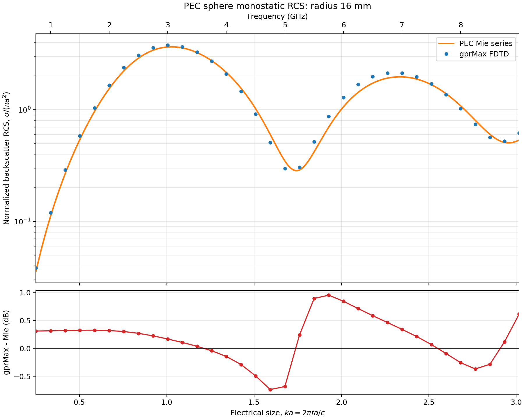
Fig. 33 Monostatic backscatter RCS from the equivalent-current NTFF output compared with the PEC-sphere Mie series over \(0.25<ka<3.02\).

For this 0.5 mm discretisation, which represents the sphere radius with 32 cells, the RMS difference over the sweep is approximately 0.44 dB. At \(ka\simeq1\), gprMax gives -25.16 dBsm and the Mie series gives -25.33 dBsm. The error grows around sharp RCS minima because a small shift in a null produces a relatively large dB difference. The principal limitation is the staircased representation of the curved PEC surface; a formal convergence study should repeat the model at several spatial resolutions and compare the complex far fields as well as RCS.

Building a heterogeneous soil

heterogeneous_soil.in

This example demonstrates how to build a more realistic soil model using a stochastic distribution of dielectric properties. A mixing model for soils proposed by Peplinski (http://dx.doi.org/10.1109/36.387598) is used to define a series of dispersive material properties for the soil.

#title: Heterogeneous soil using a stochastic distribution of dielectric properties given by a mixing model from Peplinski
#domain: 0.15 0.15 0.1
#dx_dy_dz: 0.001 0.001 0.001
#time_window: 6e-9

#waveform: ricker 1 1.5e9 my_ricker
#hertzian_dipole: y 0.045 0.075 0.085 my_ricker
#rx: 0.105 0.075 0.085

#soil_peplinski: 0.5 0.5 2.0 2.66 0.001 0.25 my_soil
#fractal_box: 0 0 0 0.15 0.15 0.070 1.5 1 1 1 50 my_soil my_soil_box
#add_surface_roughness: 0 0 0.070 0.15 0.15 0.070 1.5 1 1 0.065 0.080 my_soil_box

#geometry_view: 0 0 0 0.15 0.15 0.1 0.001 0.001 0.001 heterogeneous_soil n

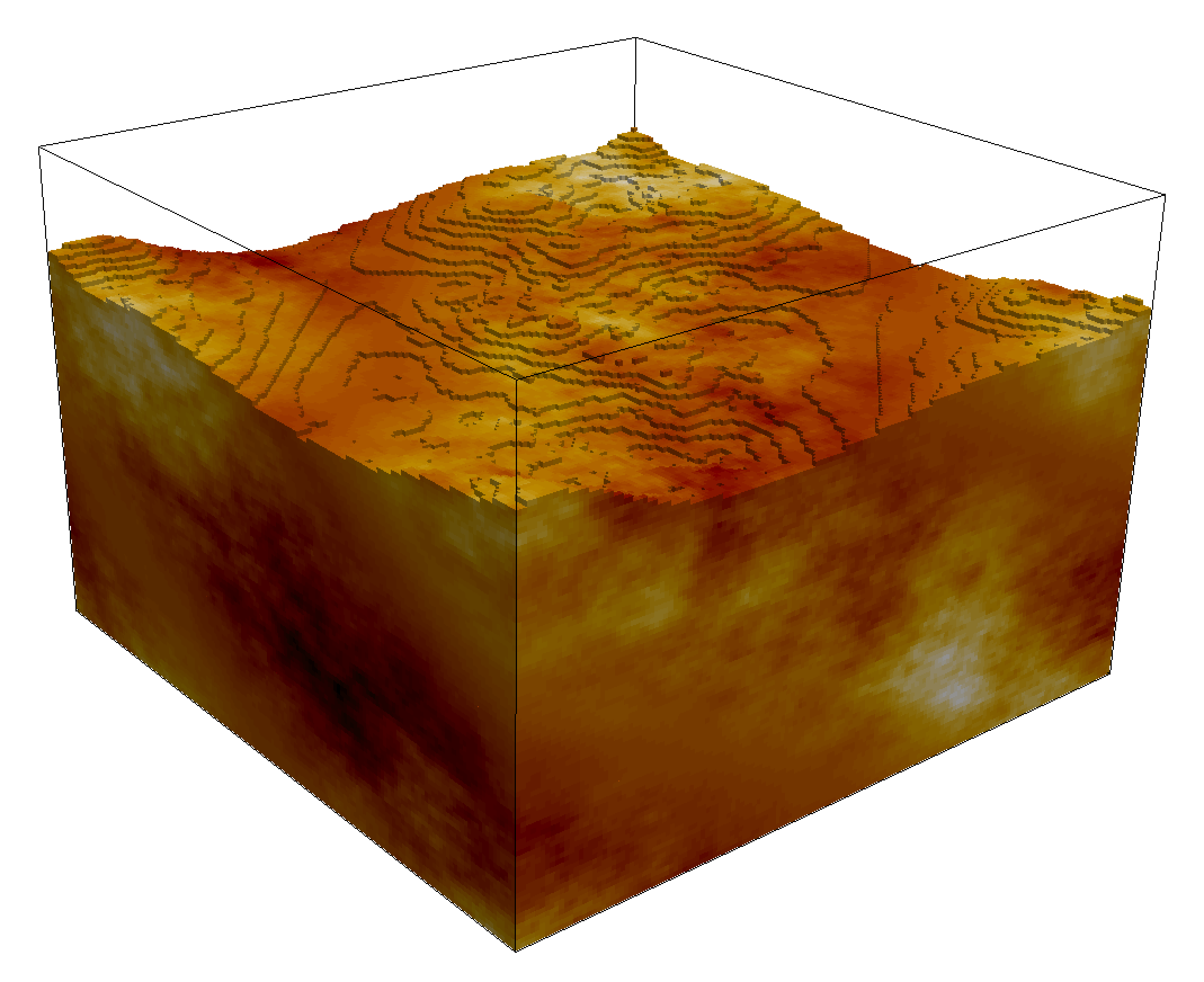
Fig. 34 FDTD geometry mesh showing a heterogeneous soil model with a rough surface.

Line 10 defines a series of dispersive materials to represent a soil with sand fraction 0.5, clay fraction 0.5, bulk density \(2~g/cm^3\), sand particle density of \(2.66~g/cm^3\), and a volumetric water fraction range of 0.001 - 0.25. The volumetric water fraction is given as a range which is what defines a series of dispersive materials.

These materials can then be distributed stochastically over a volume using the #fractal_box command. Line 11 defines a volume, a fractal dimension, a number of materials, and a mixing model to use. The fractal dimension, 1.5, controls how the materials are stochastically distributed. The fractal weightings, 1, 1, 1, weight the fractal in the x, y, and z directions. The number of materials, 50, specifies how many dispersive materials to create using the mixing model (my_soil).

Adding rough surfaces

A rough surface can be added to any side of #fractal_box using,

#add_surface_roughness: 0 0 0.070 0.15 0.15 0.070 1.5 1 1 0.065 0.080 my_soil_box

which defines one of the surfaces of the #fractal_box, a fractal dimension, and minimum and maximum values for the height of the roughness (relative to the original #fractal_box volume). In this example the roughness will be stochastically distributed with troughs up to 5mm deep, and peaks up to 10mm high.

More information, including adding surface water and vegetation, can be found in the section on using the fractal box command.

Using subgrid(s)

Including finely detailed objects or regions of high dielectric strength in FDTD modeling can dramatically increase the computational burden of the method. This is because the conditionally stable nature of the algorithm requires a minimum time step for a given spatial discretization. Thus, when the spatial discretization is lowered, either to reduce numerical dispersion or include small-sized features, the time step must be reduced. Also, the number of spatial cells is increased. One approach to reducing the overall computational cost is to introduce local finely discretized regions into a coarser finite-difference grid. This approach is known as subgridding. The computing time is reduced since there are fewer cells to solve. Also, there are fewer iterations since the coarse time step is maintained in the coarse region. gprMax uses a new Huygens subgridding (HSG) algorithm with a novel artificial loss mechanism called the switched Huygens subgridding (SHSG). For a detailed description of subgridding and the SHSG method please read [HAR2021].

Subgridding functionality requires using our Python API.

High dielectric example

cylinder_fs.py

This example is a basic demonstration of how to use subgrids. The geometry is 3D (required for any use of subgrids) and is of a water-filled (high dielectric constant) cylindrical object in freespace. The subgrid encloses the cylindrical object using a fine spatial discretisation (1mm), and a courser spatial discretisation (5mm) is used in the rest of the model (main grid). A simple Hertzian dipole source is used with a waveform shaped as the first derivative of a gaussian.

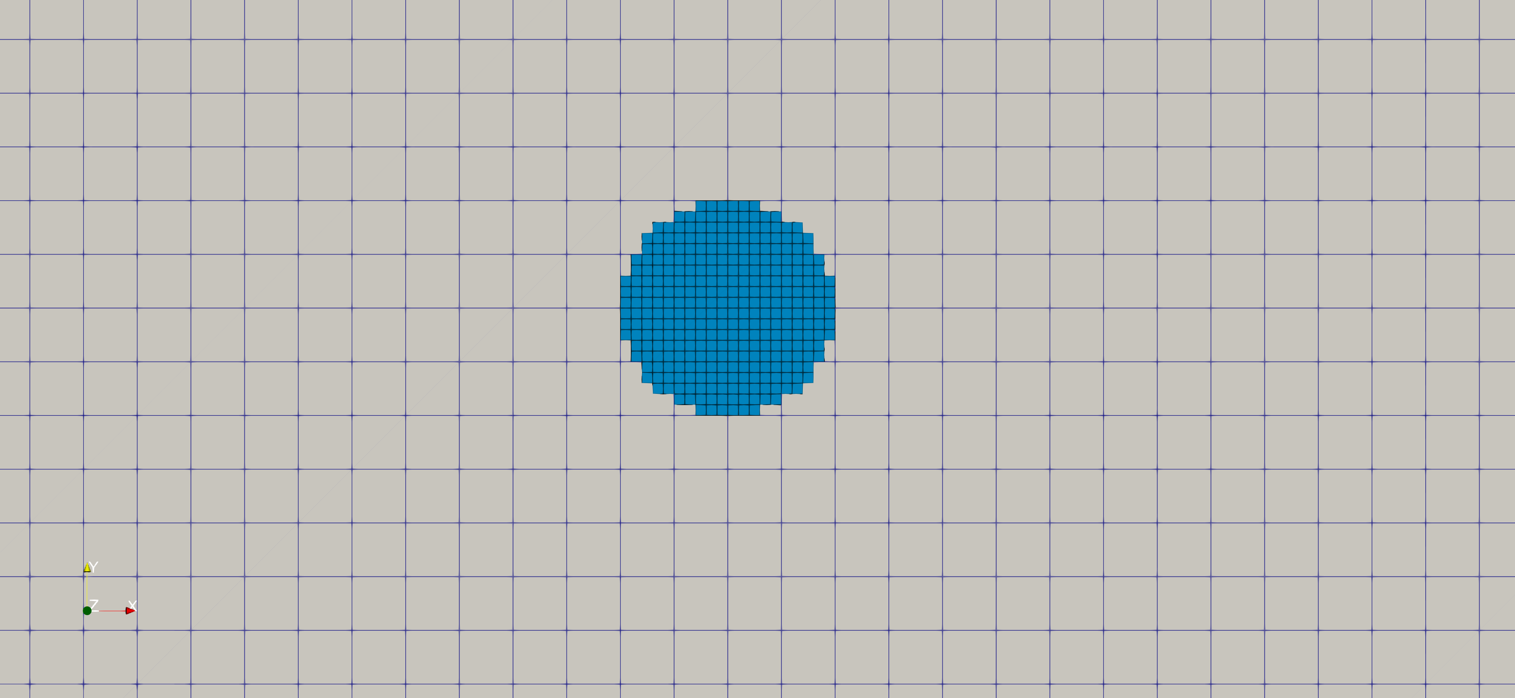
Fig. 35 The geometry of a 3D model of a water cylinder (meshed using a subgrid) in free space.

"""Cylinder in freespace

This example model demonstrates how to use subgrids at a basic level.

The geometry is 3D (required for any use of subgrids) and is of a water-filled
cylindrical object in freespace. The subgrid encloses the cylinderical object
using a fine spatial discretisation (1mm), and a courser spatial discretisation
(5mm) is used in the rest of the model (main grid). A simple Hertzian dipole
source is used with a waveform shaped as the first derivative of a gaussian.
"""

from pathlib import Path

import gprMax
from gprMax.materials import calculate_water_properties

# File path - used later to specify name of output files
fn = Path(__file__)
parts = fn.parts

# Subgrid spatial discretisation in x, y, z directions
dl_sg = 1e-3

# Subgrid ratio - must always be an odd integer multiple
ratio = 5
dl = dl_sg * ratio

# Domain extent
x = 0.500
y = 0.500
z = 0.500

# Time window
tw = 6e-9

scene = gprMax.Scene()

title = gprMax.Title(name=fn.name)
dxdydz = gprMax.Discretisation(p1=(dl, dl, dl))
domain = gprMax.Domain(p1=(x, y, z))
time_window = gprMax.TimeWindow(time=tw)

wf = gprMax.Waveform(wave_type="gaussiandot", amp=1, freq=1.5e9, id="mypulse")
hd = gprMax.HertzianDipole(polarisation="z", p1=(0.205, 0.400, 0.250), waveform_id="mypulse")
rx = gprMax.Rx(p1=(0.245, 0.400, 0.250))

scene.add(title)
scene.add(dxdydz)
scene.add(domain)
scene.add(time_window)
scene.add(wf)
scene.add(hd)
scene.add(rx)

# Cylinder parameters
c1 = (0.225, 0.250, 0.100)
c2 = (0.225, 0.250, 0.400)
r = 0.010
sg1 = (c1[0] - r, c1[1] - r, c1[2])
sg2 = (c2[0] + r, c2[1] + r, c2[2])

# Create subgrid
subgrid = gprMax.SubGridHSG(p1=sg1, p2=sg2, ratio=ratio, id="sg")
scene.add(subgrid)

# Create water material
eri, er, tau, sig = calculate_water_properties()
water = gprMax.Material(er=eri, se=sig, mr=1, sm=0, id="water")
subgrid.add(water)
water = gprMax.AddDebyeDispersion(poles=1, er_delta=[er - eri], tau=[tau], material_ids=["water"])
subgrid.add(water)

# Add cylinder to subgrid
cylinder = gprMax.Cylinder(p1=c1, p2=c2, r=r, material_id="water")
subgrid.add(cylinder)

# Create some geometry views for both subgrid and main grid
gvsg = gprMax.GeometryView(
    p1=sg1,
    p2=sg2,
    dl=(dl_sg, dl_sg, dl_sg),
    filename=fn.with_suffix("").parts[-1] + "_sg",
    output_type="n",
)
subgrid.add(gvsg)

gv1 = gprMax.GeometryView(
    p1=(0, 0, 0),
    p2=(x, y, z),
    dl=(dl, dl, dl),
    filename=fn.with_suffix("").parts[-1],
    output_type="n",
)
scene.add(gv1)

# Create some snapshots of entire domain
for i in range(5):
    s = gprMax.Snapshot(
        p1=(0, 0, 0),
        p2=(x, y, z),
        dl=(dl, dl, dl),
        time=(i + 0.5) * 1e-9,
        filename=fn.with_suffix("").parts[-1] + "_" + str(i + 1),
    )
    scene.add(s)

gprMax.run(
    scenes=[scene], n=1, geometry_only=False, outputfile=fn, subgrid=True, autotranslate=True
)

Much of the functionality demonstrated in this example is standard use of our Python API, so mainly the parts that relate to the subgrid will be described here. Lines 20-25 specify the spatial discretisation of the course main grid (5mm) and fine subgrid (1mm). Lines 56-60 specify the centres and radius of the cylinder and coordinates of a bounding box which will be used to set the domain of the subgrid.

The subgrid object is created on line 63 (providing its extent, the ratio of the spatial resolution, and a string identifier) and then added to the main scene on line 64. Any objects that are to be placed within the subgrid can be added to the subgrid scene (through the variable subgrid) in the same way as the main grid/scene.

In lines 67-71 the material used to represent water is created and added to the subgrid. The function calculate_water_properties() is used to help define the properties of water which is represented as a dispersive material using a single pole Debye model.

Lines 74-75 define a cylinder object with the material water that we just created, and then add it to the subgrid.

On lines 78-81 a view of the subgrid geometry is added to the subgrid object.

Finally, on line 95 when the model is run the keyword arguments subgrid and autotranslate are given and set to True. The subgrid argument tells gprMax that subgrids are being used, and the autotranslate argument allows the user to specify subgrid objects using main grid coordinates which will then be internally translated to local subgrid coordinates. Without using this option the user would have to specify subgrid objects in local subgrid coordinates.

Antenna modelling example

gssi_400_over_fractal_subsurface.py

This example combines an imported GPR antenna model (like a GSSI 400 MHz antenna) with a rough subsurface interface. The three-dimensional model has two soil layers: sandy soil above a higher-permittivity soil, both with conductive loss. The antenna sits on the flat ground surface at a height of 1.53 m above the model origin; the rough interface is below it.

The antenna uses its supported 2 mm spatial discretisation, preserving the contributor’s geometry and feed design. The main grid uses a 10 mm spatial discretisation, giving an odd subgrid ratio of 5. Do not remove the antenna model’s resolution check to run it on a different mesh.

The time window is chosen for the time-domain GPR response. If the automatic transmitter-port output warns about a significant late-time tail, extend the time window before using its impedance or S11 spectra; the fields need more time to decay for reliable frequency-domain processing.

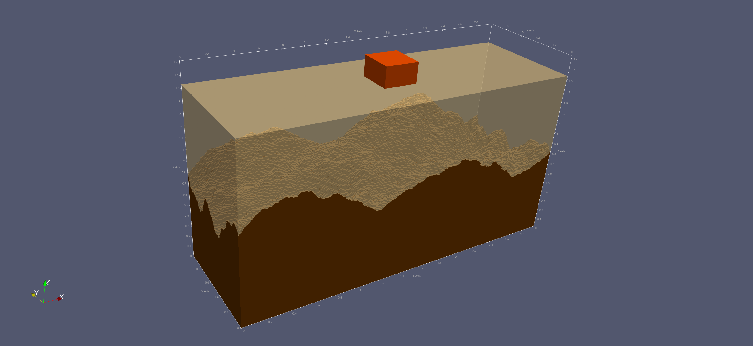
Fig. 36 Illustration of the antenna and two-layered subsurface from an earlier configuration. The downloadable example now uses a 2 mm / 10 mm mesh.

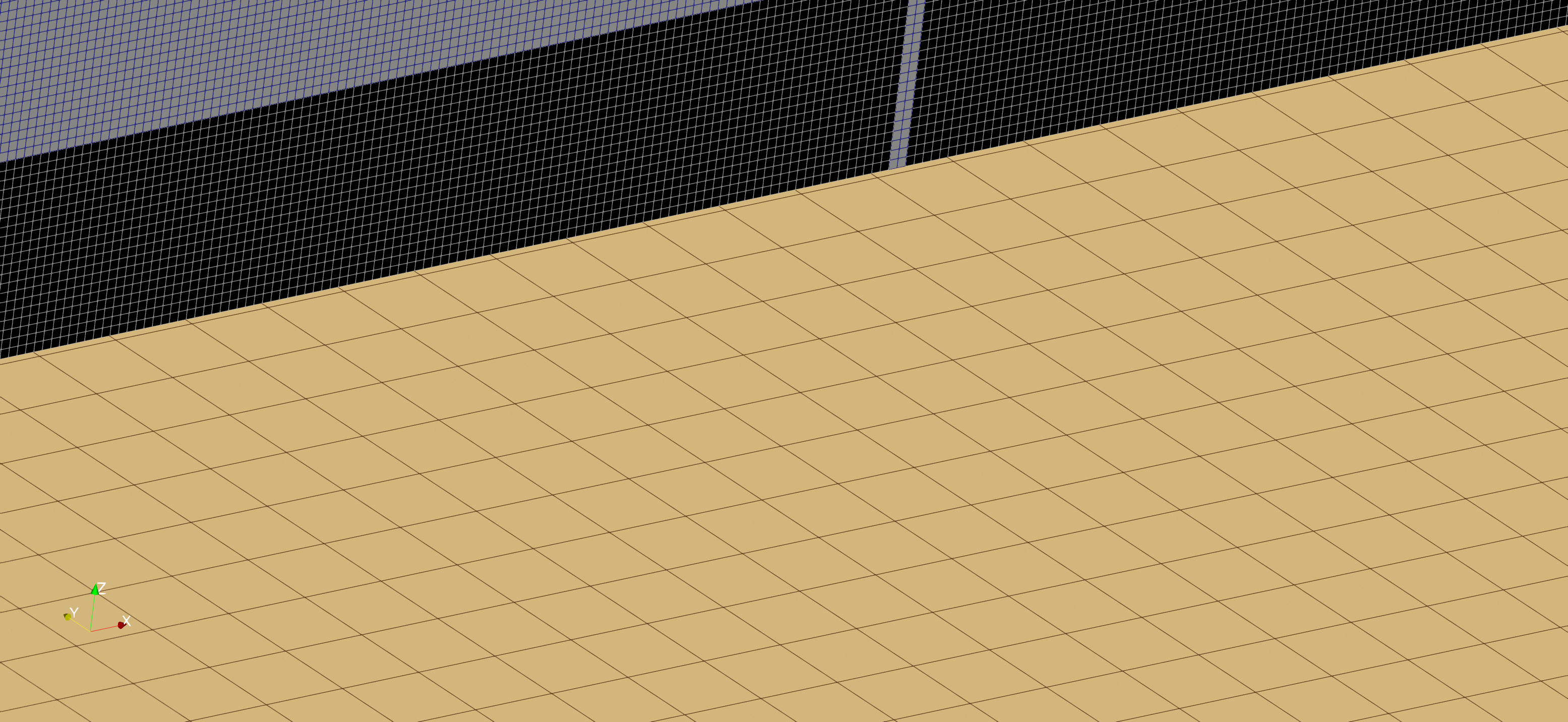
Fig. 37 Detail from the earlier 1 mm / 9 mm configuration, illustrating the subgrid placement. The current antenna example uses 2 mm / 10 mm.

"""GPR antenna model (like a GSSI 400MHz antenna) over layered media with a
    rough subsurface interface.

This example model demonstrates how to use subgrids at a more advanced level -
    combining use of an imported antenna model and rough subsurface interface.

The geometry is 3D (required for any use of subgrids) and has a two-layered
subsurface. The top layer is a sandy soil and the bottom layer a soil with
higher permittivity (both have some simple conductive loss). There is a rough
interface between the soil layers. A GPR antenna model (like a GSSI 400MHz
antenna) is imported and placed on the surface of the layered media. The antenna
is meshed using its supported 2 mm spatial discretisation, preserving the
contributor's antenna design. A coarser 10 mm spatial discretisation is used
in the rest of the model (main grid), giving a subgrid ratio of 5.
"""

from pathlib import Path

import numpy as np

import gprMax
from gprMax.toolboxes.GPRAntennaModels.GSSI import antenna_like_GSSI_400

# File path - used later to specify name of output files
fn = Path(__file__)
parts = fn.parts

# Preserve the antenna model's supported 2 mm spatial discretisation.
dl_sg = 2e-3

# Subgrid ratio - must always be an odd integer multiple
ratio = 5
dl = dl_sg * ratio

# Domain extent
x = 3
y = 1
z = 2

# Time window
# Estimated two way travel time over 1 metre in material with highest
# permittivity, slowest velocity.
tw = 2 / 3e8 * (np.sqrt(3.2) + np.sqrt(9))

scene = gprMax.Scene()

title = gprMax.Title(name=fn.name)
dxdydz = gprMax.Discretisation(p1=(dl, dl, dl))
domain = gprMax.Domain(p1=(x, y, z))
time_window = gprMax.TimeWindow(time=tw)

scene.add(title)
scene.add(dxdydz)
scene.add(domain)
scene.add(time_window)

# Dimensions of antenna case
antenna_case = (0.3, 0.3, 0.178)

# Keep the original physical soil-surface height, independent of mesh spacing.
# The antenna position is aligned with both the main grid and the subgrid.
antenna_p = (x / 2, y / 2, 1.53)

# Extra distance surrounding antenna for subgrid
bounding_box = 2 * dl

# Subgrid extent
sg_x0 = antenna_p[0] - antenna_case[0] / 2 - bounding_box
sg_y0 = antenna_p[1] - antenna_case[1] / 2 - bounding_box
sg_z0 = antenna_p[2] - bounding_box
sg_x1 = antenna_p[0] + antenna_case[0] / 2 + bounding_box
sg_y1 = antenna_p[1] + antenna_case[1] / 2 + bounding_box
# Round the antenna height up to whole main-grid cells so all inner-surface
# bounds are main-grid aligned before calculating local subgrid coordinates.
sg_z1 = antenna_p[2] + np.ceil(antenna_case[2] / dl) * dl + bounding_box

# Create subgrid
sg = gprMax.SubGridHSG(p1=[sg_x0, sg_y0, sg_z0], p2=[sg_x1, sg_y1, sg_z1], ratio=ratio, id="sg")
scene.add(sg)

# Create and add a box of homogeneous material to main grid - sandy_soil
sandy_soil = gprMax.Material(er=3.2, se=0.397e-3, mr=1, sm=0, id="sandy_soil")
scene.add(sandy_soil)
b1 = gprMax.Box(p1=(0, 0, 0), p2=(x, y, antenna_p[2]), material_id="sandy_soil")
scene.add(b1)

# Position box of sandy_soil in the subgrid.
#   It has to be positioned manually because it traverses the main grid/subgrid
#   interface. Grid traversal is when objects extend beyond the outer surface.
#   Setting autotranslate to false allows you to place objects beyond the outer
#   surface.

# Use the actual subgrid settings, including the PML and coupling padding.
ps = sg.kwargs["pml_separation"]
pc = sg.kwargs["subgrid_pml_thickness"]
isos = sg.kwargs["is_os_sep"] * ratio
padding = (ps + pc + isos) * dl_sg

# Cover the complete local grid, not just the region inside the inner surface.
soil_x = sg_x1 - sg_x0 + 2 * padding
soil_y = sg_y1 - sg_y0 + 2 * padding

# Calculate maximum z-coordinate (height) for box of sandy_soil in subgrid
h = antenna_p[2] - sg_z0 + padding

# Create and add a box of homogeneous material to subgrid - sandy_soil
sg.add(sandy_soil)
b2 = gprMax.Box(p1=(0, 0, 0), p2=(soil_x, soil_y, h), material_id="sandy_soil")
# Set autotranslate for the box object to false
b2.autotranslate = False
sg.add(b2)

# Import antenna model and add components to subgrid
gssi_objects = antenna_like_GSSI_400(*antenna_p, resolution=dl_sg)
for obj in gssi_objects:
    sg.add(obj)

# Create and add a homogeneous material with a rough surface
soil = gprMax.Material(er=9, se=0.397e-3, mr=1, sm=0, id="soil")
scene.add(soil)

fb = gprMax.FractalBox(
    p1=(0, 0, 0),
    p2=(3, 1, 1),
    frac_dim=1.5,
    weighting=(1, 1, 1),
    n_materials=1,
    mixing_model_id="soil",
    id="fbox",
    seed=1,
)
scene.add(fb)

rough_surf = gprMax.AddSurfaceRoughness(
    p1=(0, 0, 1),
    p2=(3, 1, 1),
    frac_dim=1.5,
    weighting=(1, 1),
    limits=(0.4, 1.2),
    fractal_box_id="fbox",
    seed=1,
)
scene.add(rough_surf)

# Create some snapshots and geometry views
for i in range(1, 51):
    snap = gprMax.Snapshot(
        p1=(0, y / 2, 0),
        p2=(x, y / 2 + dl, z),
        dl=(dl, dl, dl),
        filename=Path(*parts[:-1], f"{parts[-1]}_{str(i)}").name,
        time=i * tw / 50,
    )
    scene.add(snap)

gvsg = gprMax.GeometryView(
    p1=(sg_x0, sg_y0, sg_z0),
    p2=(sg_x1, sg_y1, sg_z1),
    dl=(dl_sg, dl_sg, dl_sg),
    filename=fn.with_suffix("").parts[-1] + "_sg",
    output_type="n",
)
sg.add(gvsg)

gv1 = gprMax.GeometryView(
    p1=(0, 0, 0), p2=(x, y, z), dl=(dl, dl, dl), filename=fn.with_suffix("").parts[-1], output_type="n"
)
scene.add(gv1)

gprMax.run(
    scenes=[scene], n=1, geometry_only=False, outputfile=fn, subgrid=True, autotranslate=True
)

Much of the functionality demonstrated in this example is standard use of our Python API, or covered in the introductory subgrid example earlier in this section.

The sandy-soil box inside the subgrid uses local coordinates because it crosses the interface with the main grid. Its autotranslate property is set to False. Its extent includes the coupling and PML padding, calculated from the subgrid settings rather than a fixed number of cells. The soil surface is at the same physical height in both grids. The subgrid bounds are aligned with the main grid, with the upper bound rounded upwards to contain the complete antenna.

Customising the PMLs

Through our Python API there is the ability to customise and adjust the formulation and properties used for the Perfectly Matched Layer (PML) absorbing boundaries.

Note

• If you just want to adjust the thickness of the PMLs and not use our Python API, that can be achieved using the #pml_cells command.

This example demonstrates how different formulations of PML and PML parameters can be adjusted and used.

The model is of an elongated-thin PEC plate (25 x 100 mm). The y-directed electric field (Ey) is monitored one cell away from the plate, and a z-directed Hertzian dipole source is placed diagonally opposite the field monitoring point and at 1 mm above one of the PEC sheet corner. Only three cells of free space separate the plate target from the inner surface of the PMLs.

The performance of each PML can be compared with a reference solution using the same model with a substantially larger domain.

from pathlib import Path

import numpy as np

import gprMax

# File path for output
fn = Path(__file__)
parts = fn.parts

# Discretisation
dl = 0.001

# Domain
x = 0.051
y = 0.126
z = 0.026

domain = gprMax.Domain(p1=(x, y, z))
dxdydz = gprMax.Discretisation(p1=(dl, dl, dl))
time_window = gprMax.TimeWindow(iterations=2100)
tssf = gprMax.TimeStepStabilityFactor(f=0.99)

waveform = gprMax.Waveform(wave_type="gaussiandotnorm", amp=1, freq=9.42e9, id="mypulse")
hertzian_dipole = gprMax.HertzianDipole(
    polarisation="z", p1=(0.013, 0.013, 0.014), waveform_id="mypulse"
)
rx = gprMax.Rx(p1=(0.038, 0.114, 0.013))

plate = gprMax.Plate(p1=(0.013, 0.013, 0.013), p2=(0.038, 0.113, 0.013), material_id="pec")

gv1 = gprMax.GeometryView(
    p1=(0, 0, 0),
    p2=(x, y, z),
    dl=(dl, dl, dl),
    filename=Path(*parts[:-1], f"{parts[-1]}_n"),
    output_type="n",
)
gv2 = gprMax.GeometryView(
    p1=(0, 0, 0),
    p2=(x, y, z),
    dl=(dl, dl, dl),
    filename=Path(*parts[:-1], f"{parts[-1]}_f"),
    output_type="f",
)

pmls = {
    "CFS-PML": {
        "pml": gprMax.PMLProps(formulation="HORIPML", thickness=10),
        # Parameters from http://dx.doi.org/10.1109/TAP.2018.2823864
        "pml_cfs": [
            gprMax.PMLCFS(
                alphascalingprofile="constant",
                alphascalingdirection="forward",
                alphamin=0.05,
                alphamax=0.05,
                kappascalingprofile="quartic",
                kappascalingdirection="forward",
                kappamin=1,
                kappamax=8,
                sigmascalingprofile="quartic",
                sigmascalingdirection="forward",
                sigmamin=0,
                sigmamax=1.1 * ((4 + 1) / (150 * np.pi * dl)),
            )
        ],
    },
    "HORIPML-1": {
        "pml": gprMax.PMLProps(formulation="HORIPML", thickness=10),
        # Parameters from http://dx.doi.org/10.1109/TAP.2011.2180344
        "pml_cfs": [
            gprMax.PMLCFS(
                alphascalingprofile="constant",
                alphascalingdirection="forward",
                alphamin=0,
                alphamax=0,
                kappascalingprofile="quartic",
                kappascalingdirection="forward",
                kappamin=1,
                kappamax=12,
                sigmascalingprofile="quartic",
                sigmascalingdirection="forward",
                sigmamin=0,
                sigmamax=0.7 * ((4 + 1) / (150 * np.pi * dl)),
            )
        ],
    },
    "HORIPML-2": {
        "pml": gprMax.PMLProps(formulation="HORIPML", thickness=10),
        # Parameters from http://dx.doi.org/10.1109/TAP.2018.2823864
        "pml_cfs": [
            gprMax.PMLCFS(
                alphascalingprofile="constant",
                alphascalingdirection="forward",
                alphamin=0,
                alphamax=0,
                kappascalingprofile="constant",
                kappascalingdirection="forward",
                kappamin=1,
                kappamax=1,
                sigmascalingprofile="sextic",
                sigmascalingdirection="forward",
                sigmamin=0,
                sigmamax=0.275 / (150 * np.pi * dl),
            ),
            gprMax.PMLCFS(
                alphascalingprofile="sextic",
                alphascalingdirection="forward",
                alphamin=0.07,
                alphamax=0.07 + (0.275 / (150 * np.pi * dl)),
                kappascalingprofile="cubic",
                kappascalingdirection="forward",
                kappamin=1,
                kappamax=8,
                sigmascalingprofile="quadratic",
                sigmascalingdirection="forward",
                sigmamin=0,
                sigmamax=2.75 / (150 * np.pi * dl),
            ),
        ],
    },
    "MRIPML-1": {
        "pml": gprMax.PMLProps(formulation="MRIPML", thickness=10),
        # Parameters from Antonis' MATLAB script (M3Dparams.m)
        "pml_cfs": [
            gprMax.PMLCFS(
                alphascalingprofile="constant",
                alphascalingdirection="forward",
                alphamin=0.05,
                alphamax=0.05,
                kappascalingprofile="quartic",
                kappascalingdirection="forward",
                kappamin=1,
                kappamax=8,
                sigmascalingprofile="quartic",
                sigmascalingdirection="forward",
                sigmamin=0,
                sigmamax=1.1 * ((4 + 1) / (150 * np.pi * dl)),
            )
        ],
    },
    "MRIPML-2": {
        "pml": gprMax.PMLProps(formulation="MRIPML", thickness=10),
        # Parameters from http://dx.doi.org/10.1109/TAP.2018.2823864
        "pml_cfs": [
            gprMax.PMLCFS(
                alphascalingprofile="quadratic",
                alphascalingdirection="reverse",
                alphamin=0,
                alphamax=0.15,
                kappascalingprofile="quartic",
                kappascalingdirection="forward",
                kappamin=1,
                kappamax=12,
                sigmascalingprofile="quartic",
                sigmascalingdirection="forward",
                sigmamin=0,
                sigmamax=0.65 * ((4 + 1) / (150 * np.pi * dl)),
            ),
            gprMax.PMLCFS(
                alphascalingprofile="linear",
                alphascalingdirection="reverse",
                alphamin=0.07,
                alphamax=0.8,
                kappascalingprofile="constant",
                kappascalingdirection="forward",
                kappamin=0,
                kappamax=0,
                sigmascalingprofile="quadratic",
                sigmascalingdirection="forward",
                sigmamin=0,
                sigmamax=0.65 * ((2 + 1) / (150 * np.pi * dl)),
            ),
        ],
    },
}

scenes = []
for k, v in pmls.items():
    scene = gprMax.Scene()
    title = gprMax.Title(name=fn.with_suffix("").name + "_" + k)
    scene.add(title)
    scene.add(domain)
    scene.add(dxdydz)
    scene.add(time_window)
    scene.add(tssf)
    scene.add(waveform)
    scene.add(hertzian_dipole)
    scene.add(rx)
    # scene.add(gv1)
    # scene.add(gv2)

    scene.add(v["pml"])
    for pml_cfs in v["pml_cfs"]:
        scene.add(pml_cfs)

    scenes.append(scene)

# Run model
gprMax.run(scenes=scenes, n=len(pmls), geometry_only=False, outputfile=fn)

In lines 43-122 a dictionary with different PML formulations and parameters is created.