Numerical comparisons

This section presents comparisons of models using different numerical modelling techniques.

FDTD/MoM

The Finite-Difference Time-Domain (FDTD) method from gprMax is compared with the Method of Moments (MoM) from the MATLAB antenna toolbox.

Bowtie antenna in free space

This example considers the input impedance of a planar bowtie antenna in free space. The length and height of the bowtie are 100mm, giving a flare angle of \(90^\circ\).

FDTD model

antenna_bowtie_fs.in

#python:

from gprMax.input_cmd_funcs import *

title = 'antenna_bowtie_fs'
print('#title: {}'.format(title))

domain = domain(0.200, 0.200, 0.100)
dxdydz = dx_dy_dz(0.001, 0.001, 0.001)
time_window = time_window(30e-9)
bowtie_dims = (0.050, 0.100) # Length, height
tx_pos = (domain[0]/2, domain[1]/2, domain[2]/2)

# Source excitation and type
print('#waveform: gaussian 1 1.5e9 mypulse')
print('#transmission_line: x {:g} {:g} {:g} 50 mypulse'.format(tx_pos[0], tx_pos[1], tx_pos[2]))

# Bowtie - upper x half
triangle(tx_pos[0], tx_pos[1], tx_pos[2], tx_pos[0] + bowtie_dims[0] + 2 * dxdydz[0], tx_pos[1] - bowtie_dims[1]/2, tx_pos[2], tx_pos[0] + bowtie_dims[0] + 2 * dxdydz[0], tx_pos[1] + bowtie_dims[1]/2, tx_pos[2], 0, 'pec')

# Bowtie - lower x half
triangle(tx_pos[0] + dxdydz[0], tx_pos[1], tx_pos[2], tx_pos[0] - bowtie_dims[0], tx_pos[1] - bowtie_dims[1]/2, tx_pos[2], tx_pos[0] - bowtie_dims[0], tx_pos[1] + bowtie_dims[1]/2, tx_pos[2], 0, 'pec')

# Detailed geometry view around bowtie and feed position
geometry_view(tx_pos[0] - bowtie_dims[0] - 2*dxdydz[0], tx_pos[1] - bowtie_dims[1]/2  - 2*dxdydz[1], tx_pos[2] - 2*dxdydz[2], tx_pos[0] + bowtie_dims[0] + 2*dxdydz[0], tx_pos[1] + bowtie_dims[1]/2  + 2*dxdydz[1], tx_pos[2] + 2*dxdydz[2], dxdydz[0], dxdydz[1], dxdydz[2], title + '_pcb', type='f')

#end_python:

A Gaussian waveform with a centre frequency of 1.5GHz was used to excite the antenna, which was fed by a transmission line with a characteristic impedance of 50 Ohms.

The module plot_antenna_params from the tools subpackage was used to calculate and plot the input impedance from the FDTD model.

MoM model

The bowtie antenna was created using the antenna toolbox in MATLAB, and the bowtieTriangular class.

bowtie = bowtieTriangular('Length', 0.1)
zin = impedance(bowtie, 33.33e6:33.33e6:6e9)

Results

Fig. 48 shows the input impedance (resistive and reactive) for the FDTD (gprMax) and MoM (MATLAB) models. The frequency resolution for the FFT used in both models was \(\Delta f = 33.33~MHz\).

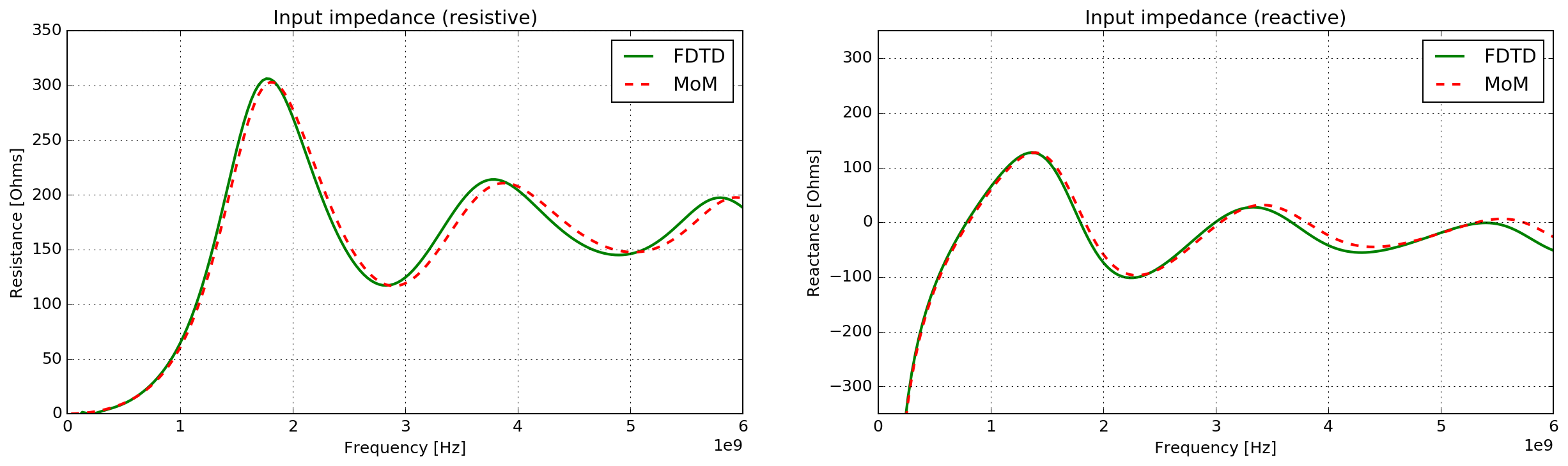
Fig. 48 Input impedance (resistive and reactive) of a bowtie antenna in free space using FDTD (gprMax) and MoM (MATLAB) models.

The results from the FDTD and MoM modelling techniques are in very good agreement. The biggest mismatch occurs in the resistive part of the input impedance at frequencies above 3GHz.