Surface impedance and impedance volumes

A surface-impedance boundary condition (SIBC) models losses in a thick conductor without meshing its skin depth. SurfaceImpedance defines the boundary response and its identifier; it does not create geometry. Assign that ID to a supported volume primitive, such as a box or sphere, to create an impedance volume. gprMax excludes fields inside the volume and applies the specified response at its voxel boundary. It does not assign the fitted bulk conductivity to interior cells and solve the fields inside the metal.

This is a closed, electrically opaque volume, not a transmissive sheet. Choose it for thick conductors with a local scalar surface response. A one-cell-thick volume still blocks transmission; it does not become a thin film model. The presets describe smooth, non-magnetic bulk metal at 293 K, not roughness, plating, temperature dependence, or optical materials.

This guide starts with setup and result checks. The equations and validation evidence are in Surface impedance: theory and validation.

The published HTML guide renders the shared parameter table that GitHub’s source preview cannot expand.

First copper model

The existing rectangular-waveguide example compares identical PEC and copper guides. It is a useful first check for someone accustomed to assigning a finite-conductivity wall in a frequency-domain simulator.

The following defines the surface model and geometry for that workflow. It assumes scene already contains a domain and mesh, and lower/upper are the corners of a finite-thickness wall; the runnable script below supplies them. Lengths are in metres, frequencies in Hz, and conductivity in S/m.

scene.add(gprMax.SurfaceImpedance(
    id="copper_wall", preset="copper",
    fit_frequency_range=(80e9, 200e9),
    fit_order="auto", fit_tolerance=2e-3, plot_fit=True,
))
scene.add(gprMax.Box(
    p1=lower, p2=upper, material_id="copper_wall", averaging="n",
))

The model measures 130–150 GHz. The wider 80–200 GHz fit covers its pulse and modal anchors; a fit band is the range over which the boundary model is accurate, not the list of output frequencies. gprMax also checks the discrete-time response at the modal anchor frequencies. If that check reports an out-of-band frequency, follow frequency is outside ... fit band rather than ignoring the warning or forcing a lower fit order.

With gprMax installed in the active Python environment, run from the repository root:

python examples/features/impedance_surface/rectangular_waveguide_comparison/run_comparison.py --geometry-only
python examples/features/impedance_surface/rectangular_waveguide_comparison/run_comparison.py
python examples/features/impedance_surface/rectangular_waveguide_comparison/plot_results.py

The first command builds the voxel geometry and solves the transverse modal fields without advancing time. Inspect the copper fit PNG and both *_eigenmode_fields.png files beside the script. Check the intended TE10 pattern and confinement before running the second command.

The full comparison writes pec_rectangular_waveguide.h5 and copper_rectangular_waveguide.h5. The plotter writes rectangular_waveguide_eigenmode_comparison.png and prints the 140 GHz effective indices, copper attenuation, and wall-to-centre electric-field ratios. Expect a small tangential electric field at the copper wall and zero at the PEC wall. Copper’s passive forward effective index has negative imaginary part, corresponding to positive attenuation.

FDTD launches a pulse and records its evolution. This example deliberately stops its walls before PML and uses a short record before wall-end reflections return. It demonstrates the local wall law, not a matched termination. For a longer transmission experiment, use the uniform PML or virtual-guide setup in Waveguides and absorbers. Independently scaled modal pictures show shape; use the receiver ratios and complex effective index for quantitative comparisons.

Choosing a surface model

Table 9 SurfaceImpedance arguments

Argument	Default	Meaning and constraints
id	Required	Unique material identifier used by geometry. Shares the bulk-material namespace; do not use + or the reserved __impedance_ prefix.
preset	None	Named thick-metal model. Choose exactly one of preset, conductivity, or resistance.
conductivity	None	Positive finite bulk conductivity in S/m, fitted to a good-conductor surface response. This is not a resistance in ohms.
resistance	None	Positive surface resistance in ohms, or positive infinity for exact voxel-face PMC. Zero, negative values, NaN, and negative infinity are invalid; use PEC for a zero-impedance wall.
fit_frequency_range	Required for a fit	Positive finite increasing (fmin, fmax) in Hz. Required with preset or conductivity; unavailable with resistance. Cover the excitation and modal solve range, including the discrete-frequency check explained in the guide.
fit_order	"auto"	Select the smallest runtime pole count from 1 through 64 meeting the tolerance. An integer from 1 through 64 requests that exact count; if the tolerance is not met, gprMax issues a warning rather than changing the count.
fit_tolerance	2e-3	Positive finite relative impedance-fit tolerance (0.2% by default). Automatic fitting must meet it; explicit-order fitting issues a warning if it is not met.
plot_fit	False	Write a fit PNG in geometry-only runs. True also writes it during full runs. Neither setting opens a window. Only available for fitted models.

Metal presets and bulk conductivity

Available presets are aluminium, copper, gold, molybdenum, palladium, silver, tungsten, and zinc. Case-insensitive element symbols and aluminum are also accepted. Use a supplied conductivity when you have a suitable bulk value instead of a named preset:

scene.add(gprMax.SurfaceImpedance(
    id="custom_wall", conductivity=3.2e7,
    fit_frequency_range=(8e9, 12e9), fit_order="auto",
))

Both routes fit the same passive good-conductor model. Fitted bands cannot exceed 300 GHz and must satisfy the good-conductor applicability check. The model assumes the real conductor is several skin depths thick. These checks and the fit construction are derived in Common-metal Foster presets.

The selected pole count is available as fit_pole_count and fit_result.selected_pole_count. More poles cost memory and update time; the automatic setting avoids an unnecessarily high order for a narrow band. For example, automatic fitting selects two poles over 8–12 GHz at the default tolerance. State-space coefficients are internal and cannot be supplied to the public constructor. They are saved for reproducibility in Surface-impedance reproducibility metadata.

Ideal resistance and exact PMC

Use a constant resistance for an idealised boundary experiment:

scene.add(gprMax.SurfaceImpedance(id="resistive_wall", resistance=50.0))
scene.add(gprMax.SurfaceImpedance(id="pmc_wall", resistance=float("inf")))

Assign either ID to the same kind of opaque volume geometry as copper. A frequency-independent real resistance is not the dispersive surface response of a physical metal; gprMax reports that limitation when it is built.

Positive infinite resistance gives exactly zero surface admittance and is the PMC boundary at the main-voxel face. It does not approximate infinity with a large finite number. Built-in pmc volume geometry uses legacy H constraints that can move a flat wall’s effective reflection plane by half a cell. Its use, including PMC-equivalent materials, warns once per affected grid. Unused declarations, internal TE constraints, and PMC symmetry planes do not trigger that geometry warning. See Exact voxel-face PMC for the exact update and reflection-plane validation.

Equivalent hash commands

The same surface models and geometry can be specified with hash commands:

#surface_impedance: copper_wall preset copper 80e9 200e9 auto 2e-3 y
#surface_impedance: custom_wall conductivity 3.2e7 8e9 12e9
#surface_impedance: resistive_wall resistance 50
#surface_impedance: pmc_wall resistance inf
#box: 0.10 0.07 0.05 0.20 0.13 0.10 copper_wall n

These are definitions and a geometry fragment, not a complete input file. For fitted surfaces, the optional final y enables fit plots during full runs as well as geometry-only runs. The default, n, writes fit plots only during geometry-only runs. See Model Building for the full command syntax and Advanced Model Building (Python API) for the Python constructor reference.

Building geometry

Geometry follows declaration order: later objects overwrite earlier ones. Several primitives with the same surface-impedance ID can form a body; a later air or dielectric object can cut a cavity. Tags are optional metadata, not a way to assign impedance. The final voxel geometry determines which faces receive the boundary law. Refine curved or oblique walls until both their staircase representation and the result of interest converge; avoiding skin-depth cells does not remove the need to resolve the surrounding fields and geometry.

Supported geometry

Surface-impedance IDs can be assigned directly to boxes, spheres, ellipsoids, cylinders and cones (axis-aligned or oblique), finite-thickness cylindrical sectors, and finite-thickness triangular prisms. Their final voxel boundaries must satisfy the connectivity checks described below. A FractalBox can also use a surface-impedance ID as its mixing_model_id, but it must set n_materials=1 because one opaque volume cannot contain a graded set of surface models, and it must be used with a roughness, grass, or water modifier. For an unmodified single-material volume, use Box instead.

Assign one scalar surface-impedance model, not a different model for each direction. In the Python API, use material_id rather than directional material_ids. Hash-command geometry must likewise use the surface-impedance ID as its sole material identifier. Surface-impedance geometry is not dielectric-smoothed.

Plates, electric or magnetic edges, zero-thickness triangles and cylindrical sectors, and boxes that collapse to zero cells on any axis are rejected. Those sheet and line objects have retained fields on both sides and require a two-sided sheet transition condition rather than the implemented one-sided opaque-volume boundary.

Impedance geometry cannot currently be exported and reimported using GeometryObjectsWrite and GeometryObjectsRead. Recreate the SurfaceImpedance definition and native geometry in the destination scene.

The volume must occupy at least one cell along every non-empty axis and there must be at least one retained cell between the complete impedance region and each non-symmetry domain boundary. The region may extend to a declared PEC or PMC symmetry plane, or continue uniformly through a longitudinal PML to its outer boundary, subject to the requirements in Waveguides and absorbers.

Voxel-boundary topology

The final voxel geometry, after all drawing and cutout operations, must have an unambiguous boundary. Cells belonging to one body must meet through full faces, not only through an edge or corner. Both the opaque body and the surrounding retained field region must remain locally connected. Separate bodies are allowed; a contact between different surface-impedance IDs is still checked as part of the same excluded geometry, with no surface response on an internal metal-to-metal face.

When an error identifies a bad edge or vertex, inspect that part of the voxel model. Thicken a narrow connection, separate touching bodies, refine the mesh, or shift a curved surface relative to the grid. Two individually valid primitives can produce an invalid union or cutout. The exact local quadrant tests are in Discrete geometry and contacts.

Contacts and symmetry

Isotropic PEC, PMC, and impedance volumes may touch. PEC forces a shared tangential electric component to zero regardless of adjacent-object drawing order. A diagonal PEC/SIBC contact with separating retained cells produces a warning; face-sharing contacts do not. Use isotropic materials: directional PEC/PMC mixtures at an impedance boundary are rejected.

Legacy PMC contacts keep their existing reflection-plane limitation. They do not turn an adjacent impedance surface into an exact PMC. For a wall at the voxel face, use infinite surface resistance as described above.

PEC and PMC SymmetryBoundary planes are supported on all six domain faces, including intersecting planes. The geometry must also be valid after reflection across the symmetry plane. No artificial end cap is introduced where the excluded volume meets it. See Discrete geometry and contacts for the component constraints and retained-area treatment.

Run the contact example to inspect its geometry and contact-field traces:

python examples/features/impedance_surface/pec_pmc_contacts.py --output-dir results/contacts
python examples/features/impedance_surface/pec_pmc_contacts.py --symmetry pmc --output-dir results/symmetry

Use --symmetry pec for the corresponding PEC plane.

Two-dimensional models

Use DomainMode(mode="TE") or DomainMode(mode="TM") and float("inf") for the domain’s invariant extent. Extrude the impedance geometry through that entire dimension. gprMax supports all three choices of invariant axis; the geometry cannot vary across its synthetic storage layers. Those layers do not represent a physical thickness. Modal power in 2D is reported per metre along the invariant direction.

Running reliably

Automatic time-step margin

FDTD advances fields in small time steps. The mesh imposes a maximum Courant–Friedrichs–Lewy (CFL) time step; the usual stability-factor command scales that limit. Declaring any SurfaceImpedance caps the factor at 0.99, preserving a smaller user setting. It does not multiply a factor of 0.8 by 0.99: the result remains 0.8.

The cap applies before time windows and sources are built, even for an unused surface declaration. If it reduces the requested factor, the build log explains the change and reports the effective time step. Geometry reuse does not apply the cap twice, and the original Scene objects are unchanged. Models without a surface declaration keep their ordinary time-step behaviour.

To request more margin, use the existing command:

scene.add(gprMax.TimeStepStabilityFactor(f=0.9))

The equivalent hash command is #time_step_stability_factor: 0.9. A time window in seconds keeps its duration and adjusts the iteration count. A window specified as an iteration count instead becomes shorter in physical time. Use the same explicit factor in comparative PEC runs if samples must share the same physical times.

The cap addresses sensitivity near the CFL endpoint; it is not a general stability guarantee. In particular, it does not repair the invalid custom PML profiles discussed below. See Clipped-circulation stability for the clipped-circulation analysis and long-run evidence.

Mesh, bandwidth, and recording time

Check convergence separately in mesh spacing, fit accuracy, modal anchors, and recording duration. The pulse must fit within the time window and the response must have time to decay. A longer record can reveal a late return from a reflecting termination that a short record hides. Extra output frequency bins alone do not improve any of these approximations.

Supported solver configurations

The implementation supports three-dimensional and two-dimensional main-grid CPU models. All TE and TM invariant-axis orientations are supported. The following combinations are deliberately rejected:

• CUDA, OpenCL, and Metal field solvers;

• MPI domain decomposition and subgrids;

• thin wires in the same grid;

• an impedance boundary which changes along a PML absorption direction;

• a lumped electric source, rational-network terminal, or transmission-line edge which overlaps a boundary electric edge;

• a directional PEC/PMC material mixture immediately outside the boundary.

An axial discrete plane wave is unsupported because it samples the completed geometry to construct its layered auxiliary line. A homogeneous vector/angle discrete plane wave is supported only when the complete impedance boundary is strictly inside its total-field/scattered-field box.

A direct gprMax.EigenmodePort in 3D or 2D may cross an impedance guide. The guide boundary must be invariant along the propagation direction through both cells adjacent to the modal plane. Every port window has a PEC transverse boundary, whether or not a VirtualWaveguide is attached. Tangential electric fields on the rim are zero. This constraint replaces complete SIBC rows on the rim as well as rows whose magnetic stencil would extend outside the window, so the modal solve and auxiliary guide use the same boundary condition. The build reports when this replaces surface rows. To retain a wall’s surface impedance and loss, extend the window at least one opaque voxel beyond it. The interior rows keep their magnetic circulation, bulk mass, surface admittance, and histories; missing samples in these rows are still rejected. A guide end cap normal to the propagation axis cannot cross the retained solve region.

The window may cut across a ground plane or another uniformly extruded impedance volume. This is an artificial PEC truncation, not an open boundary or a continuation of the metal beyond the window. Enlarge the window to check convergence of the mode and S-parameters, especially where appreciable fields reach its edges. Opaque padding remains useful when the whole guide fits within the window.

Choosing an SIBC eigenmode port window

The drawings below show cross-sections looking along the propagation axis. Place the port plane perpendicular to the guide, on a section where both the retained medium and SIBC wall continue unchanged on either side. The dashed rectangle is the modal window; it is not a change to the physical geometry. The examples use propagation along z, but the same rule applies to other port normals.

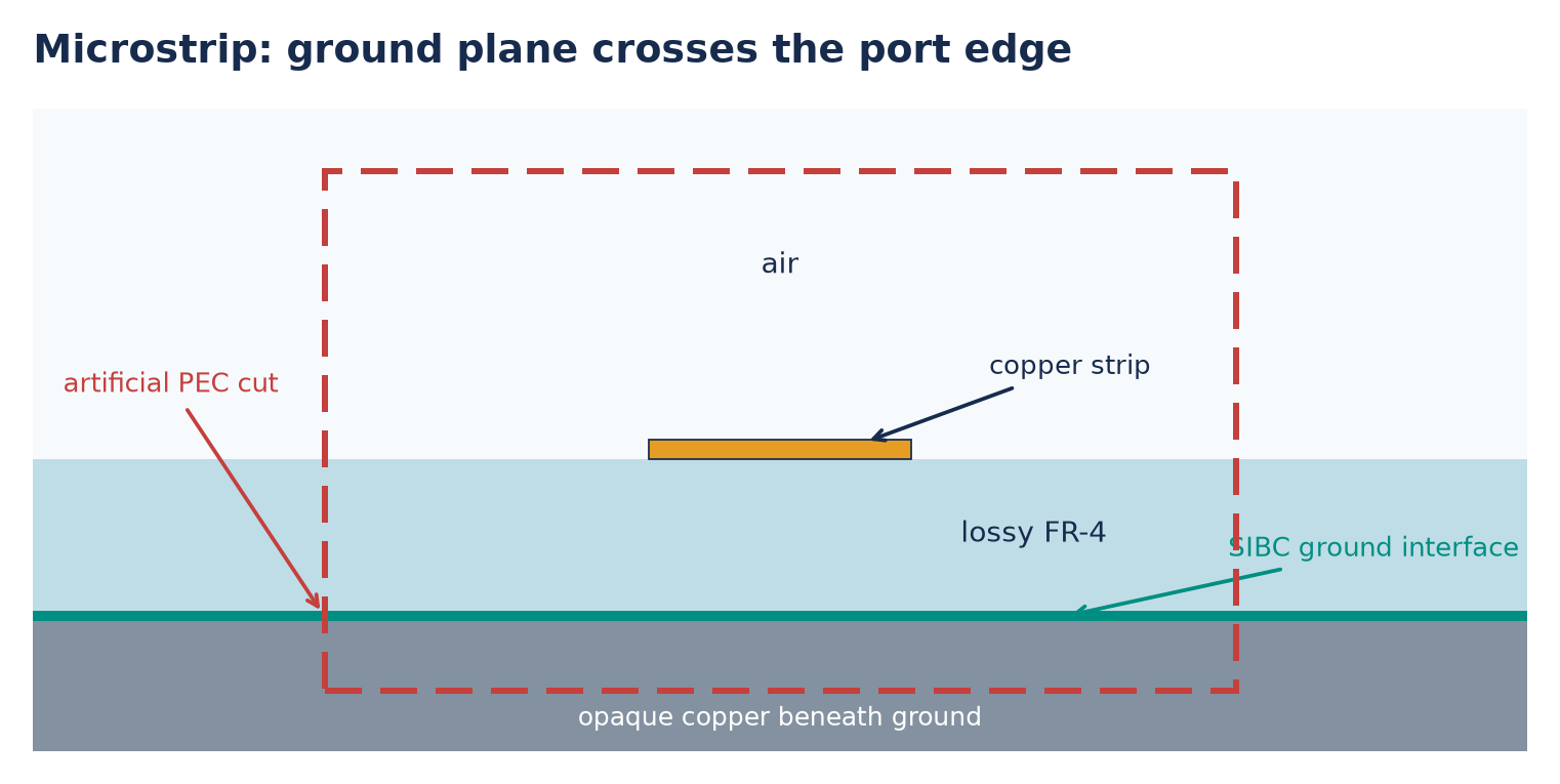
Fig. 6 Microstrip. Include the strip, substrate, and significant fringing field. The window can cut the extended SIBC ground plane at its side edges. Those cropped surface rows meet the artificial PEC port boundary; the ground interface and lossy FR-4 within the aperture remain physical. The opaque copper below the ground keeps the ground interface inside the window, preserving its SIBC loss.

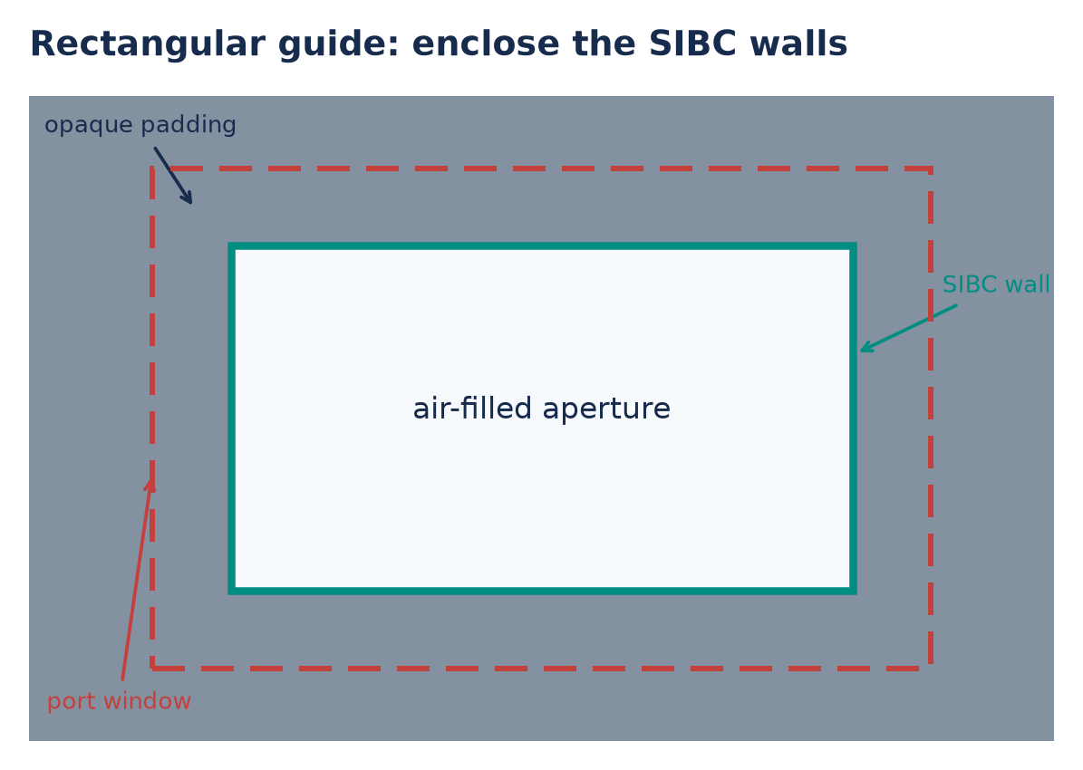
Fig. 7 Rectangular waveguide. Put the entire air aperture and all four SIBC walls inside the window. Extend the window at least one opaque voxel past every wall to retain its surface impedance in the modal solve and, when attached, the auxiliary PML. If a wall lies exactly on the rim, it becomes PEC in the modal solve and virtual guide, removing that wall’s impedance and loss from the modeled continuation.

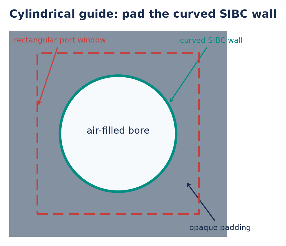
Fig. 8 Cylindrical waveguide. Enclose the circular bore and its SIBC wall in the rectangular modal window, with opaque voxels outside the wall to keep it inside the PEC rim. The circle is schematic: the solver sees a voxelized wall. Refine the transverse grid and check the mode and S-parameters for convergence, especially near the curved boundary.

Waveguides and absorbers

A port launches and measures a wave; it does not absorb a returning wave. Either extend the physical guide into domain PML or attach a VirtualWaveguide: a matched termination to its port. The eigenmode guide explains the setup, port directions, and active/passive choices. The additional SIBC requirements are collected here:

• Keep the wall and the surrounding host medium uniformly extruded along every intersecting PML absorption direction, including neighbouring stencil cells. Wall faces must be tangent to that direction; end caps, steps, and changes of surface model inside the absorber are rejected.

• At the intersecting edges, retained bulk materials may be heterogeneous, lossy, and electrically dispersive (Debye, Lorentz, Drude, or inclusive mixtures). Each must be isotropic, with positive finite high-frequency permittivity and permeability and finite nonnegative conductivities. Air/substrate junctions are supported. Each constituent must continue unchanged through the absorber and its neighbouring stencil cells. The surface itself may also be dispersive.

• Both HORIPML and MRIPML support one or two CFS terms for this coupling. For an internal PMLSlab, extend its transverse bounds into the opaque volume to cover the wall’s electric and magnetic samples. Ending a bound exactly on the wall can omit required samples and is rejected.

• A virtual-guide modal window may intersect SIBC walls at its artificial PEC rim. The modal solve and auxiliary guide both clamp tangential electric fields there, including on complete physical SIBC walls at the rim. Use opaque padding beyond a wall to retain its surface impedance. In 2D these constraints apply only along the physical transverse axis, not the synthetic invariant dimension. CPU virtual guides support the same lossy/dispersive retained hosts as domain PML, including independent bulk and surface histories at the aperture and throughout the auxiliary absorber.

• Keep the existing source clearance and fit-band requirements. SIBC coupling is available on CPU main grids in 3D and all TE/TM orientations, in either propagation direction; it does not support subgrids, MPI, or accelerator solvers.

Boundary PMLs may carry the uniformly extruded volume to the outer domain boundary without a retained-cell gap there. The virtual guide copies the aperture and its surface model into a separate auxiliary grid; you do not draw that continuation in the main geometry.

Try the executable reduced-mode examples:

python examples/features/impedance_surface/virtual_waveguide_2d.py --mode TM --wall pmc
python examples/features/impedance_surface/virtual_waveguide_2d.py --mode TE --wall foster

The source and auxiliary surface histories receive the coupled boundary correction, including for exact PMC. The update equations and comparisons with physical continuations are in PML and virtual-guide coupling.

A copper microstrip with air above a lossy or dispersive substrate may continue into longitudinal domain PML with the same cross-section. The strip and ground must occupy finite-thickness voxels and extend through the absorber; keep their transverse end faces clear of transverse PML. For dispersive substrates, DispersiveAveraging(enabled=True) makes the bulk interface sampling consistent with the surface solver’s retained-area integration. A pulse comparison with a causally longer line is available as:

python -m testing.validation.impedance_surface.validate_microstrip_pml --host all

Custom PML errors

The demonstrated unstable second-order HORIPML product profiles are rejected during coefficient construction. The error identifies the profile and the offending electric or magnetic sample. Reducing the time step does not cure this profile instability. Use one CFS factor, or apply the specific second-alpha repair described in Selecting a stable second-order HORIPML profile for the investigated unit-kappa, unshifted-first-factor configuration. The repair matches the second alpha grading to 1.1 * sigma1; it is not a universal recipe for arbitrary profiles.

Keep explicit zero conductivity distinct from automatic conductivity: None requests automatic selection. Passing the profile guard does not certify stability for every material and geometry combination.

Results and troubleshooting

Use the fit plot to check the surface model over its fit band, modal plots to check the field pattern, and modal coefficients or receiver traces to check the simulated response. These answer different questions. The HDF5 surface metadata records the chosen model and discrete-time coefficients; see Surface-impedance reproducibility metadata. For modal S-parameters, also apply the validity masks explained in Reading coefficients and validity.

non-passive on the discrete band

The trapezoidal unit-circle response has negative real impedance. This is an internal fit failure for the public passive models and should be reported with the input and fit band.

frequency is outside ... fit band

Expand the preset or conductivity fit band to include every eigenmode anchor frequency and its bilinear-warped frequency. Close to Nyquist the warped frequency can be much higher than the physical anchor. Reducing dt also reduces the difference.

impedance-volume voxel topology is non-manifold at a Yee edge

The error reports the edge orientation and grid index where two impedance quadrants touch only diagonally. Connect the impedance cells through a full voxel face, or move them apart so they no longer share the reported edge. Refining the mesh, thickening the feature, increasing a curved object’s radius, or adjusting its position can change the final rasterization.

impedance-volume voxel topology is non-manifold at grid vertex

The error reports the vertex index and whether the impedance cells, retained cells, or both are not face-connected within its incident 2 x 2 x 2 neighbourhood. Reshape the geometry so both sets connect through voxel faces, or separate the impedance regions so they share neither an edge nor a vertex. The check includes contacts between different surface-impedance IDs.

must have at least one retained cell or PML intersection

Move or shorten the impedance volume. The excluded region can touch only declared PEC or PMC symmetry faces of the domain, or continue uniformly through a longitudinal PML. Check the extrusion, host-material, and slab coverage requirements in Waveguides and absorbers for a PML intersection.

eigenmodes require a propagation-invariant boundary

Move the modal plane into a uniform section, extend the guide through both adjacent normal cells, remove an end cap at the plane, and make the modal window include the complete aperture.

Unexpected gain or positive Im(n_eff)

Check the \(e^{+j\omega t}\) and \(e^{-j\beta w}\) conventions, the metal-to-dielectric normal, fit passivity, and forward-mode selection. For the implemented convention, a passive forward mode has \(\operatorname{Im}n_{\mathrm{eff}}<0\).

Large source-plane reflection

Confirm that source and monitor anchors cover the significant waveform band, the guide is uniform at the source plane, wall-end returns are outside the measurement gate, and the modal window is large enough that its artificial PEC rim does not affect the guided mode. Then refine the Yee grid and repeat. Do not infer boundary failure from a trace contaminated by a nearby open guide end.

Metal result disagrees with measurement

Check temperature, purity, alloying, plating thickness, surface roughness, magnetic permeability, and whether several skin depths fit inside the real conductor. The preset is a local semi-infinite good-conductor model, not a universal named-material database.

See also

Surface impedance: theory and validation contains the boundary and ADE equations, clipped-field update, stability analysis, and validation evidence.