Impulse-response waveform synthesis

Information

Use --receiver name:label:Ez (or study:id:Ez) for numbering-independent selection. A selected subset retains original receiver paths and identity metadata, so receiver numbers can have gaps. See Receiver numbering and cross-version processing.

This toolbox uses one impulse-excited gprMax model to generate receiver histories for many different source pulses. It is useful when the geometry, materials, source type, and receiver arrangement remain fixed, but the source waveform must be varied. The expensive FDTD solution is then run once; the additional pulses require only post-processing.

For a linear, time-invariant discrete FDTD model,

\[y_x[n]=(h*x)[n]=\sum_m h[n-m]x[m],\]

where \(x[n]\) is the scalar driving waveform, \(h[n]\) is the discrete transfer response between that source and a receiver, and \(y_x[n]\) is the receiver output. If the reference source contains the one-sample impulse

\[x_\delta[n]=A\delta[n-n_\delta],\]

then its stored receiver output is

\[y_\delta[n]=A h[n-n_\delta].\]

The toolbox therefore calculates each requested output directly from the stored impulse run:

\[y_x[n]=\frac{1}{A}\sum_m y_\delta[n+n_\delta-m]x[m].\]

It reads \(A\) and \(n_\delta\) from the actual source samples; it does not assume a continuous-time unit-area Dirac delta or that the impulse must occur at array index zero. The full causal convolution is formed before it is cropped to the original receiver time window.

The method is exact, to floating-point precision, for the same discrete linear FDTD system. It includes linear dispersive materials, PMLs, and all multiple scattering already present in the impulse response. It is the general waveform form of the impulse-response principle used by the SFCW toolbox.

Timing

The target waveform must be sampled on the same update lattice as the reference source. gprMax output records both:

• TimeSampleOffset – the physical Yee time associated with a stored driving sample; and

• WaveformEvaluationTimeOffset – the time at which the waveform function was evaluated during that update.

These are identical for current local sources. A hard voltage source prescribes \(E^0\) before the first observation and then \(E^{n+1}\) using the waveform at \((n+1)\Delta t\); both offsets are zero. Its sample-zero impulse is therefore retained in the measured response.

Older hard-source files have an evaluation offset of zero but a physical offset of \(\Delta t\). The toolbox uses each file’s evaluation offset when constructing target samples and retains its physical offset in the output. Older files without the evaluation attribute are handled using the source type and driving quantity; do not manually relabel their time axes.

A zero-valued hard waveform still clamps the feed while the source is active. An impulse reference and a directly driven model must use the same feed boundary condition. Removing the impulse clamp is not equivalent to leaving a hard voltage source in place for subsequent waveform synthesis.

The output receiver samples retain their original electric, magnetic, or current Yee-time offset. No additional half-step phase correction is needed.

Preparing an impulse model

Use one active scalar source with the built-in impulse waveform. The source position, type, resistance or network, polarisation, start time, geometry, and materials must be those required in every synthesised model. Only the waveform may change.

The supplied example contains a PEC cylinder in a dielectric half-space:

Download the impulse-response example.

#waveform: impulse 1 1 impulse
#hertzian_dipole: z 0.200 0.320 inf impulse
#rx: 0.240 0.320 inf response Ez

Run it normally:

python -m gprMax \
    gprMax/toolboxes/ImpulseResponse/examples/cylinder_impulse_2D.in

The reference must contain exactly one significant source sample. The toolbox also rejects another active scalar source because its contribution cannot be separated from the selected impulse response. Multiple-source superposition can instead be performed from one separate impulse run per source.

Command-line usage

Inspect the stored sources and receiver components:

python -m gprMax.toolboxes.ImpulseResponse inspect cylinder_impulse_2D.h5

Generate two built-in gprMax pulses from that one run:

python -m gprMax.toolboxes.ImpulseResponse process cylinder_impulse_2D.h5 \
    --source /srcs/src1 \
    --waveform ricker 1 500e6 ricker_500MHz \
    --waveform gaussian 1 350e6 gaussian_350MHz \
    --receiver /rxs/rx1:Ez \
    --stop-time 20e-9 \
    --max-frequency 1.2e9 \
    --output-dir cylinder_waveforms \
    --plot cylinder_waveforms.png

The four values after --waveform follow the familiar gprMax order: waveform type, amplitude, frequency in hertz, and identifier. The option may be repeated. All current built-in waveform definitions are supported. If --receiver is omitted, every stored E, H, and requested I receiver component is processed. Merged B-scans are convolved along their time axis; use --source-file to identify an original A-scan containing the source history when the merged file does not contain it.

--start-time and --stop-time apply common activation times to all built-in waveforms in a command. The stop time is particularly useful for a finite-duration contsine. Sampled CSV columns end naturally when their time column ends and therefore ignore --stop-time.

Arbitrary sampled waveforms

One CSV file can contain several user pulses. Its first column must be time in seconds and every remaining column name becomes a waveform identifier:

time,measured_pulse,alternative_pulse
0.0,0.0,0.0
1.0e-11,0.12,0.04
2.0e-11,0.31,0.15
...

Use it with:

python -m gprMax.toolboxes.ImpulseResponse process cylinder_impulse_2D.h5 \
    --waveform-file measured_pulses.csv \
    --output-dir measured_waveforms

The columns contain the same scalar driving quantity and units reported for the reference source, for example amperes for a Hertzian electric dipole or volts for a voltage source. They are linearly interpolated at the exact source waveform-evaluation times and set to zero outside the CSV time range. --start-time applies a common source start time to built-in and CSV waveforms.

Python API

The processing functions can be used directly:

from gprMax.toolboxes.ImpulseResponse import (
    load_source_sampling,
    sample_builtin_waveform,
    synthesise_output,
    write_synthesised_output,
)

source = load_source_sampling("cylinder_impulse_2D.h5", "/srcs/src1")
pulse = sample_builtin_waveform(
    source,
    "ricker",
    amplitude=1,
    frequency=500e6,
    waveform_id="ricker_500MHz",
)
result = synthesise_output(
    "cylinder_impulse_2D.h5",
    pulse,
    receiver_selections=[("/rxs/rx1", "Ez")],
    valid_max_frequency=1.2e9,
)
write_synthesised_output("cylinder_ricker_500MHz.h5", result)

Output

One HDF5 file is written for each target waveform. It preserves the selected receiver paths, dataset timing attributes, and root grid metadata so ordinary receiver plotting tools can read it. The selected source path contains the new target samples and waveform metadata. /impulse_reference records the original impulse samples and provenance.

These are waveform-synthesis products, not complete reruns. They contain the selected receiver histories only. Snapshots, NTFF fields, derived S-parameters, antenna metrics, and other state-dependent outputs are not regenerated.

Finite records and numerical bandwidth

The impulse run must be long enough to contain every physical arrival needed in the new waveforms. The toolbox reports the peak in the final five percent of each impulse receiver relative to its overall peak. A high tail means that cropping assumes a non-negligible missing response. Extend the FDTD time window whenever possible. --tail-taper FRACTION is available for a carefully inspected residual numerical tail, but it also suppresses genuine late arrivals within that interval.

An FDTD impulse has energy up to Nyquist, but the spatial mesh is not accurate over that entire range. --max-frequency records a user-selected numerical validity limit and reports the fraction of each target waveform’s discrete spectral energy above it. It does not silently filter the waveform. Choose the limit using the shortest wavelength and material properties in the model, normally requiring at least ten cells per wavelength.

The diagnostic counts both members of each positive/negative FFT-frequency pair. DC and, for an even sample count, the Nyquist bin are counted once. Only bins strictly above the limit contribute to the numerator, and an all-zero waveform reports zero. The ratio is therefore the fraction of the finite real waveform’s discrete energy in those bins, not an error estimate for the FDTD solution. Rescaling the waveform does not change that fraction.

End-to-end verification

The implementation was tested using a 2D PEC-cylinder scattering model in double precision. One impulse run was used to synthesise 500 MHz Ricker, 350 MHz Gaussian, and 450 MHz normalised Gaussian-derivative receiver histories. Each was compared with a separate FDTD run using that waveform directly.

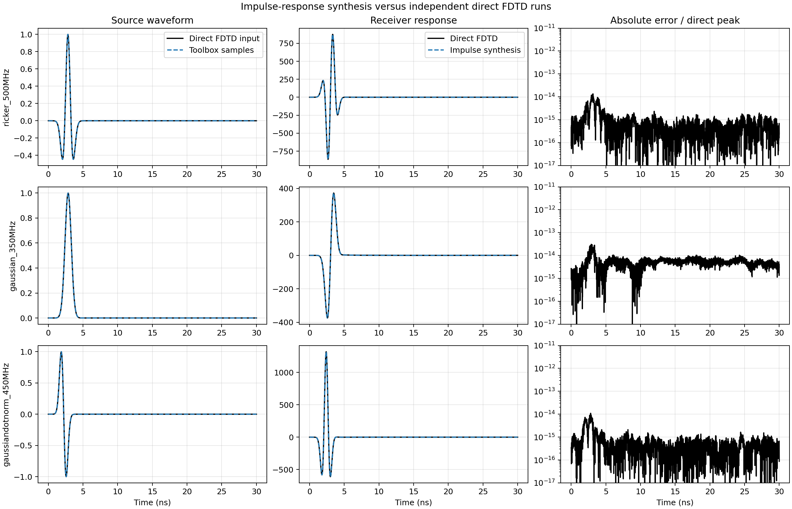
Fig. 87 Built-in target samples and receiver histories from impulse synthesis compared with independent direct FDTD runs. The right column shows the absolute sample error normalised by the corresponding direct-trace peak.

The maximum receiver errors were \(1.35\times10^{-14}\) for the Ricker, \(3.08\times10^{-14}\) for the Gaussian, and \(1.10\times10^{-14}\) for the normalised Gaussian derivative. These are double-precision round-off levels. The reproducible driver is testing/regression/impulse_response/validate_waveform_synthesis.py; a smaller end-to-end version is included in the automated test suite.

Limitations

• The geometry, materials, boundary conditions, source implementation, and receiver arrangement must not change between target waveforms.

• The model and source coupling must remain linear and time invariant.

• One impulse run characterises one active source. Array excitations require one impulse response per independently driven element followed by linear superposition with the desired amplitudes and delays.

• A different source type or source resistance requires a new impulse run.

• Only stored receiver quantities are synthesised; solver-internal fields and derived output objects cannot be reconstructed from point receivers.