Eigenmode tracking guide
Mode tracking connects independently solved port fields into a consistent broadband field bank. It follows branches through crossings, aligns phase, and selects reproducible bases for degenerate groups. This guide covers the inputs, workflow, automatic symmetry selection, and inspection of the resulting fields. For aperture setup and S-parameter measurement, see Eigenmode ports and S-parameter analysis; for equations and implementation details, see Eigenmode tracking theory.
On this page
Enabling tracking and choosing what to inspect
Add tracking="auto" to each participating source and receiver port.
This also enables symmetry detection and basis selection for eligible
degenerate groups on supported 3D port cross sections. Explicit
mode_polarizations takes precedence when selecting a pair’s directions.
Start with the default verification="full" when evaluating a model.
verification="fast" skips the extra mesh and window solves, so it provides
less evidence about box modes. Examples 8 and 9 use fast to keep their
inspection runs short; change it to full to perform those extra checks.
scene.add(gprMax.EigenmodePort(
    port=1, p1=(0.02, 0.005, 0), p2=(0.02, 0.075, float("inf")),
    direction="+", modes=(1, 2), anchors="auto",
    tracking="auto", verification="full", plot_fields=True,
))
anchors="auto" and tracking="auto" do different jobs: anchors choose
where to solve; tracking chooses which solutions to connect. You can also
provide an explicit list of anchor frequencies, as Examples 8 and 9 do.
Mode labels are assigned at the anchor nearest the band center (the lower
frequency on a tie), then followed toward both ends of the band. Thus
mode=1 means a tracked channel, not necessarily the first raw solution at
every frequency. When comparing with an older run, check the actual fields
at both ports rather than assuming that the same number means the same
polarization.
Run Examples 8 and 9 with --geometry-only to inspect their dispersion
curves and modal fields before the time-domain simulation. Their scripts set
plot_fields=True, so a full run also produces these plots. At a crossing,
check that the labels follow consistent fields. For TE11, check that the chosen
polarizations stay aligned. For an open guide, check the outer-edge fields and
any confinement warnings. Read the warning status as well as the curve: a
smooth curve can still describe a questionable profile.
Tracking does not guarantee low S11. Correctly matched fields can still be interpolated too coarsely, especially near cutoff. Check convergence with closer anchor spacing, a suitable aperture, mesh resolution, PML thickness, and recording duration when small reflections matter.
Tracking input arguments
Pass these arguments to gprMax.EigenmodePort. The aperture, propagation
direction, and port identifier are configured as in Eigenmode ports and S-parameter analysis.
The first table covers channel selection and basis construction; the next
table lists every EigenmodeTrackingConfig control.
Argument |
Default |
Use |
|---|---|---|
|
Required |
Public channel indices, or a positive integer count. With automatic tracking these labels refer to the anchor nearest the band center, then follow the matched fields. Internal partners do not add public channels. |
|
|
Frequencies in Hz at which to solve the port. Accepts a positive frequency, an increasing sequence, or automatic selection. Tracking may add midpoint solves to resolve ambiguous associations. |
|
|
|
|
|
With automatic tracking, |
|
|
An |
|
|
Optional single transverse axis or real three-vector. Its orthogonal partner is inferred using the positive port normal. Applied after subgroup resolution with automatic tracking, or to declared pairs with legacy tracking. Shared direction pairs in either tracker and legacy mode/group mappings are deprecated and will be removed in gprMax 5.0. |
|
|
Legacy groups such as |
|
|
|
Symmetry detection and basis selection run automatically with tracking="auto"
on supported 3D port cross sections. Legacy tracking skips symmetry selection.
Polarization vectors use the Python API. Keep the same basis convention
at both ports when comparing their channel coefficients.
Advanced thresholds and limits
Most users can leave these settings at their defaults. Inspect the fields and
geometry before relaxing a threshold to suppress a warning. Pass
tracking_config=gprMax.EigenmodeTrackingConfig(...) or a mapping to
override the defaults below. Omitted fields keep their defaults. All thresholds
are dimensionless; integer controls count candidates, refinement steps, or
additional solves. These controls apply only to automatic tracking.
Thresholds must be finite and in (0, 1]; extra_candidates and
max_depth are nonnegative integers, and max_solves is a positive integer.
Parameter |
Default |
Meaning |
|---|---|---|
|
|
Common maximum relative residual for input eigenpairs, mixed reduced vectors, and available reconstructed-field checks. Eigenvalue-gap, propagation, and power checks also apply. |
|
|
Maximum normalized propagation-constant drift in mesh/window verification. |
|
|
Minimum squared field overlap, or smallest squared principal subspace overlap, in verification comparisons. |
|
|
Maximum fraction of the squared E/H field norm in the outer edge strip (10% of each transverse extent, at least one cell) used as confinement evidence at artificial boundaries. |
|
|
Minimum squared field/subspace overlap for a candidate match. This is distinct from the stricter verification overlap. |
|
|
Minimum total-cost advantage over an alternative one-to-one assignment for an individual-mode match. |
|
|
Minimum separation of the squared projection scores of the last selected and first excluded members when extracting a subgroup from a larger cluster. |
|
|
Cost of leaving an individual mode unmatched rather than forcing a poor match. |
|
|
Relative eigenvalue gap for candidate clusters. It does not relax the stricter |
|
|
Additional internal eigenpairs requested per solve, subject to solver size, to find competing branches or missing partners. |
|
|
Maximum adaptive midpoint-refinement steps for resolving identity ambiguity; |
|
|
Stop refining an ambiguous interval when its width divided by its midpoint frequency reaches this threshold. |
|
|
Budget for additional adaptive and verification solves per port. Required primary anchors are retained independently of this budget. |
For example, allow more internal candidates while retaining all other defaults:
tracking_config = gprMax.EigenmodeTrackingConfig(extra_candidates=6)
# Pass tracking="auto", tracking_config=tracking_config to EigenmodePort.
Compared with released 4.0.1, the general residual default increases from
1e-8 to 1e-7. Mixed-mode acceptance now uses this setting instead of
the previous fixed 1e-9 limit, including legacy degenerate groups. Set
residual_tolerance=1e-9 to retain that mixed-mode limit; this also tightens
the other residual checks. See Eigenmode tracking theory for the
additional reconstructed Maxwell-residual checks.
The equivalent hash options use the field names directly, without a
tracking_config prefix:
#eigenmode_port: 1 0.02 0.005 0 0.02 0.075 inf + 1,2 auto y tracking=auto verification=full extra_candidates=6
How automatic tracking works
An anchor is a frequency at which the port eigenproblem is solved. A candidate is one of that solve’s eigenmodes. A branch is the sequence of fields associated across anchors. A degenerate group contains independent fields with the same propagation constant; its individual eigenvectors can rotate while their combined span stays unchanged.
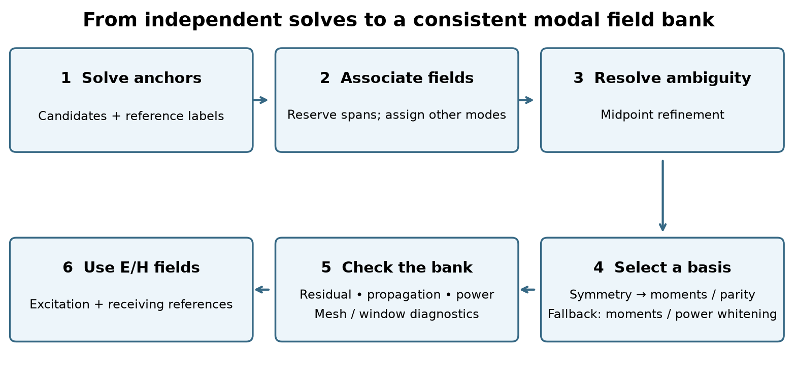
Fig. 17 Association establishes continuity; basis selection supplies reproducible E/H fields for interpolation. Extra candidates and midpoint solves help resolve ambiguous matches.
Solve and seed labels. Solve the primary anchors with extra internal candidates. Assign public labels at the anchor nearest the band center, and work outward toward lower and higher frequencies.
Associate fields. For isolated modes, combine E/H overlap and eigenvalue prediction in a global one-to-one assignment. Degenerate candidates are recognized and reserved by span matching before this individual assignment. When a group encounters another branch or group, projection and continuity tests identify the persistent subgroups inside the enlarged cluster.
Refine ambiguous intervals. Insert midpoint anchors when overlap or assignment margins cannot resolve a match. Refinement stops at the configured depth, frequency spacing, or solve budget; unresolved intervals retain their diagnostic status.
Construct a reproducible basis. Align each isolated mode’s common E/H phase. For a persistent degenerate group, field mixing means applying the same linear combination to all E and H components. Verify the discrete symmetry, separate longitudinal-field families, and resolve irreducible subspaces. Electric moments or mirror parity orient each doublet; directional field variation separates compatible equal-parity singlets. The fallback retains a power-whitened basis for the full group. An explicit direction is applied afterward within each eligible doublet. No waveguide preset or mode-index template is required.
Check and use the bank. Record identity, residual, propagation, power, and boundary diagnostics separately. Eligible propagating fields supply excitation. Receiving references can also describe evanescent fields, with finite normalization and valid coefficient decomposition.
Power whitening transforms the group’s full real-power matrix to the identity. Consequently a coefficient vector has power equal to its squared norm, and unitary changes of basis preserve that power. It supplies a stable numerical basis when a physical orientation cannot be determined.
After physical families are separated, whitening is applied within each retained block. Cross-block power terms are retained: the complete bank’s power is evaluated with its full Hermitian power matrix.
The candidate-cluster gap and the mixing tolerance serve different purposes.
cluster_gap searches for nearby branches; the stricter eigenvalue-spread
and residual checks decide whether their fields may be combined. Increasing
cluster_gap alone does not enable approximate mixing of split modes.
Why track modes?
A broadband pulse contains many frequencies. To launch the intended mode across that band, the port needs to know what its field looks like at each frequency. It solves the fields at a set of frequencies called anchors, then interpolates between them.
That interpolation only makes sense if the anchor fields belong together. Blending an x-polarized mode at one frequency with an unrelated y-polarized mode at the next creates the wrong broadband source, even if both individual mode solves are accurate. It can also make the receiving port measure the wrong channel. Mode tracking decides which fields belong to the same mode as frequency changes. Its verification checks also warn about profiles that may be distorted by the finite port aperture.
When mode numbers swap: a crossing in an anisotropic guide
An anisotropic dielectric can affect x- and y-polarized fields differently. Their propagation constants can therefore cross as frequency changes, as in Worked simulation: branch crossing in a square anisotropic guide. The fields remain distinguishable, but their order in the solver’s list changes. For example:
Frequency |
First solution in the sorted list |
Second solution in the sorted list |
|---|---|---|
Below a crossing |
Mostly x-polarized |
Mostly y-polarized |
Above the crossing |
Mostly y-polarized |
Mostly x-polarized |
If the source simply took the first solution at every anchor, its polarization would switch at the crossing. Interpolating those fields would blend two different channels. A receiver using the same mistaken numbering could then report an apparent change in transmission or coupling between modes.
Automatic tracking compares the field patterns, as well as how their propagation constants change. In this example it connects the x-like field below the crossing to the x-like field above it, even when its raw solution number changes. The selected channel follows one curve through the crossing instead of jumping to the other curve. Distinct modes retain their own propagation constants; tracking does not average them together.
In the plots, follow one label across neighbouring frequencies: its field should change consistently. A crossing in the dispersion plot is not itself an error. At an avoided crossing, the physical fields can gradually exchange character; tracking is not a rule that forces every mode to stay x-polarized or y-polarized forever.
When polarization rotates arbitrarily: the circular TE11 pair
A circular waveguide has two TE11 modes with the same propagation constant. One can be chosen x-polarized and the other y-polarized. Because they are degenerate (they share that propagation constant), rotated combinations are equally valid solutions.
An eigensolver might return x/y fields at one anchor and two diagonal fields at the next. Nothing in the circular guide has rotated: the solver has simply chosen different representatives of the same pair. Interpolating the first returned field at each frequency would make the source polarization vary across the pulse’s band. Measured coupling into the other polarization could then reflect this choice of fields rather than a physical effect.
Automatic tracking recognizes the pair and aligns it as a pair. In
Worked simulation: the circular TE11 pair, it chooses x/y directions consistently at the
anchors, so a selected input polarization keeps its meaning across the band.
The pair does not need to be declared with degenerate, and
mode_polarizations is optional. Supply "y" when you want y/-x
directions instead of x/y, and use the same choice at both ports.
Even if you request only modes=(1,), the tracker can solve the second member
internally to align the pair. That extra solve does not add another public
input or output channel. Alignment is only allowed when the modes really can
be mixed without breaking their field equations. Two nearby modes with
different, resolved propagation constants stay separate.
When the mode belongs to the artificial box
An open guide, such as a coplanar waveguide, has fields extending into the surrounding air. The mode solver can only see the finite cross-section inside the port aperture. Its artificial outer boundary can influence the fields or support a pattern that mainly belongs to that calculation box. This is a box mode; it is not the same as a legitimate mode confined by the physical metal walls of a waveguide.
A box mode can be solved very accurately and still be a poor representation of the intended guide. If used for injection or measurement, it can produce results that depend strongly on the chosen aperture. Following that pattern consistently across frequency would not, by itself, make it a good profile.
With verification="full", automatic tracking asks practical questions:
Is much of the field still present near the artificial outer boundary?
If the window is enlarged using the surrounding model geometry, does the field pattern or propagation constant change appreciably?
Does a finer transverse grid give a consistent result?
These checks can flag a suspected box mode or poorly confined profile. Mesh sensitivity alone does not prove that a mode is a box artifact. Nor can the checks always distinguish an artificial mode from a real guided mode whose field has simply been cut off by a small aperture.
For example, a low-frequency CPW mode can have a wide field extending far into the air. A small aperture may truncate it and trigger a warning, even though it is the intended mode. A confinement or box-mode warning does not remove the profile: it remains available if its numerical solution, tracking, and forward power are valid. The warning says that accuracy may be reduced. Enlarge the aperture, leave enough surrounding non-PML geometry for the checks, and compare the fields and S-parameters. Tracking helps identify the problem; it cannot supply the missing space around the guide.
Degeneracy and polarization choices
What degeneracy means for a port
Two modes are degenerate when they have the same propagation constant at a given frequency but independent field patterns. They accumulate the same propagation phase along a uniform guide. This does not mean that they are duplicate results or that only one should be kept: they represent two independent channels that the guide can carry.
The circular TE11 pair is a familiar example. An ideal circular guide has no preferred transverse direction. One TE11 pattern can be oriented with its overall electric polarization along y and another along x. Rotated combinations, such as two diagonal polarizations, describe the same pair equally well. The chosen pair of patterns is called a basis. Changing the basis changes how we label and combine the channels, not the guide.
Why mode numbers alone can be misleading
An eigensolver finds valid field patterns, but symmetry does not tell it which one to call vertical. At one frequency it might return vertical and horizontal patterns as modes 1 and 2; at another it might return the same patterns in reverse order, or two diagonal combinations. Small numerical differences can change that choice even when the physical guide is unchanged. This is a change of basis, not evidence that the guide has converted the wave’s polarization.
Broadband ports solve several frequency anchors and interpolate their fields. If mode 1 means vertical at one anchor and diagonal at the next, interpolating those raw patterns would change the intended polarization across the pulse spectrum. Tracking the complete degenerate pair lets gprMax compare the same two-channel space before choosing its labels.
Which option should I use?
Use
degenerate=(1, 2)when you want the pair tracked together but do not need mode numbers to mean particular physical directions with legacy tracking. Its initial basis is arbitrary; subsequent anchors follow it smoothly.Also use
mode_polarizations="y"when you want mode 1 to mean vertical and mode 2 horizontal for a z-directed guide. gprMax enforces those physical directions independently at each retained anchor. Use the same assignments at the receiving port to measure the same labels.Use
tracking="auto"to detect groups and select their bases through symmetry, electric moments, and mirror parity. The fundamental circular pair selects transverse directions as in Worked simulation: the circular TE11 pair.degenerateis ignored in this mode;mode_polarizationsremains useful for rotating or swapping the default directions.
Declaring the pair neither excites both channels nor forces their physical
propagation constants to become equal. EigenmodeExcitation still selects
the channel to launch. A declared pair contributes two channels to a complete
S-matrix study, so each needs its own independent excitation case.
Near equality alone is not enough to justify mixing. For example, an elliptical guide can split the circular pair into modes with different propagation constants. Those modes accumulate different phases, and a combination can change polarization as it travels. That is physical beating, which should be represented using independent modes. gprMax accepts exact or numerically unresolved degeneracy for mixing. It rejects resolved splitting in a declared group and keeps split automatic branches separate; the thresholds and alignment method are in Degenerate subspaces and physical alignment.
Physically labeled degenerate modes
The default mode_polarizations=None uses automatic basis selection.
Supply one transverse axis ("x", "y", or "z") or one real
three-vector such as (1, 1, 0) to orient every eligible doublet. The first
channel follows that direction; the second follows the positive port-normal
axis crossed with it. For a z-normal port, "y" gives y/-x. This convention
is independent of propagation sign. Use the same setting at both ports.
With tracking="auto", the complete parent group is tracked and subdivided
by longitudinal content, symmetry, and directional variation first. The
requested direction is then applied independently inside each resolved
two-dimensional block. Singlets remain unchanged: two accidentally degenerate
singlets are not combined into a polarization pair. If symmetry selection is
unavailable, an entire two-mode parent can be oriented when its integrated
electric moments are independent; larger unresolved parents cannot.
With tracking="legacy", the direction applies to the declared two-mode
pairs, without automatic symmetry selection. In either mode, a request with
no eligible pair or a pair with zero or ill-conditioned integrated transverse
E raises an error. Higher-order doublets with vanishing moments retain their
automatic mirror-based orientation when the option is omitted.
First and second refer to the lower and higher tracked indices inside the
resolved pair, including any internally retained partner. The direction must
be finite, nonzero, real, and transverse. It is normalized; a normalized normal
component above 1e-12 is rejected. The inferred partner is orthogonal.
Deprecated since version Unreleased: Two-direction sequences remain supported with both tracking="legacy"
and tracking="auto", preserving both requested directions and signs,
including valid nonorthogonal pairs. Per-mode/per-group mappings require
legacy tracking. These compatibility forms emit a visible FutureWarning
and will be removed in the next major release, gprMax 5.0.
Prefer one global direction for every pair: it keeps channel orientation
consistent and avoids separate mode/group settings. The second direction is
inferred as the positive port normal crossed with the first direction.
For example, migrate mode_polarizations=("y", "x") or
mode_polarizations={1: "y", 2: "x"} to mode_polarizations="y" for a
z-normal port. The inferred partner is -x, so this migration changes the
second channel’s phase by 180 degrees relative to an explicit +x reference.
Use the same convention at both ports when comparing complex S-parameters.
With legacy tracking, the compatibility forms require declared two-mode
degenerate pairs. With automatic tracking, a shared direction pair is
applied inside each eligible doublet after automatic subgroup selection:
# Deprecated compatibility forms: each emits a warning.
mode_polarizations=("y", "x")       # Shared explicit pair.
mode_polarizations={1: "y", 2: "x"} # Directions for both members.
mode_polarizations={(1, 2): "y"}    # One direction for this declared pair.

# Preferred form for legacy and automatic tracking.
mode_polarizations="y"             # Shared y/-x pair for a z-normal port.
In hash input, the corresponding deprecated values are
mode_polarizations=y;x, mode_polarizations=1:y;2:x, and
mode_polarizations=1,2:y. Replace them with mode_polarizations=y.
Explicit direction pairs must be transverse and independent, with a
condition number no greater than 10. Nonorthogonal pairs cannot be represented
by one direction; retain the explicit pair through the deprecation period
when that basis is required. Legacy mappings may orient selected declared
pairs while leaving the others to generic subspace alignment; incomplete or
overlapping mappings raise an error.
For circular TE11 propagating along z, assign the channels once:
scene.add(gprMax.EigenmodePort(
    port=1, p1=(0, 0, 0.02), p2=(0.05, 0.05, 0.02), direction="+",
    modes=(1, 2), anchors="auto", tracking="auto",
    mode_polarizations="y",  # The partner is automatically -x.
))
scene.add(gprMax.EigenmodeExcitation(port=1, mode=1, waveform="auto"))
Here mode 1 is vertically polarized (global y); changing only mode=1 to
mode=2 launches horizontal polarization (global -x). Reversing propagation
does not change these electric-field labels. anchors="auto" selects the
frequency anchors; it does not enable automatic mode tracking. Set
tracking="auto" explicitly to discover pairs without degenerate.
Equivalent hash options follow the existing anchor and plotting arguments:
## One direction for every detected pair:
#eigenmode_port: 1 0 0 0.02 0.05 0.05 0.02 + 1,2 auto tracking=auto mode_polarizations=y
## One diagonal direction; its orthogonal partner is inferred:
#eigenmode_port: 1 0 0 0.02 0.05 0.05 0.02 + 1,2 auto tracking=auto mode_polarizations=1,1,0
Use one definition per port and no spaces inside hash option values. Omitting
the option corresponds to Python None. Semicolon-separated directions and
colon-based mappings raise an error. Values are parsed without expression
evaluation.
Polarization describes the direction of the transverse electric field
integrated across the aperture; local arrows need not all be parallel. gprMax
aligns that direction at every retained frequency anchor. Geometry-only plots,
single-anchor and broadband sources, monitors, studies, and virtual guides
all use the same aligned fields. Set plot_fields=True to also write the
standard modal pictures during a full run. Example 7 shows the two tracked
TE11 profiles.
With only degenerate, the group is tracked smoothly, but its orientations
at the reference anchor remain arbitrary. With neither argument, modes keep
the existing independent tracking. Physical axis/vector selection requires
a two-mode group in a 3D cross-section. With one direction, the second is inferred.
Declare a group only for exact or numerically unresolved degeneracy. If asymmetry resolves the splitting, excite the independently solved modes or correct unintended geometry asymmetry. A group with negligible integrated electric field cannot be oriented by axis/vector references; use generic group tracking. These failures and their numerical thresholds are derived in Degenerate subspaces and physical alignment.
Automatic symmetry detection
With tracking="auto", no symmetry label is required. EigenmodePort detects C4v or
C2v from the discretized port at every solved anchor and uses the strongest
group common to the bank. C4v requires a square mesh with equal spacing;
C2v requires the two grid-axis mirrors and also applies to rectangular meshes.
The tests compare complex diagonal material tensors and PEC/PMC masks about
the port-window center (relative tolerance 1e-10, absolute 1e-12).
Resolved eigenvalues remain separate tracking branches.
Native rotations and reflections act on the complete staggered E/H fields.
Their modal representations must preserve each eligible span and its power
metric, and satisfy the group relations before decomposition. Centered
circular and octagonal interfaces can preserve C4v after staircasing; a
hexagonal interface can retain C2v. C4v produces singlets or E doublets;
C2v produces singlets. C2v labels use the port normal as the twofold axis,
with B1 u-like and B2 v-like under the two mirrors.
The algorithm supports any group dimension: repeated C4v doublets can produce
2+2+2 from a six-dimensional span or ten doublets from a twenty-dimensional
span. One-dimensional representations remain single channels. Frequency
continuation aligns the resulting blocks across the active anchor range.
Repeated copies of the same symmetry can contain different field families. The code first compares longitudinal electric and magnetic content through a small generalized eigenproblem. In a uniform metallic guide this separates TE and TM copies. In a dielectric guide it supplies a field-based family selection when the longitudinal scores are distinct. Singular or unresolved scores retain the existing symmetry decomposition.
Within each native doublet, the code first tries to align the integrated
transverse electric moments with the u and v axes. It uses a unitary polar
factor to preserve whitened power, accepting moments with relative strength
above 1e-12, condition number below 1e8, and the expected vector
mirror parities. If this test fails, diagonalizing the u-mirror selects its
odd and even partners, in that order. The v-mirror supplies an independent
parity check. Reflections act on E as a polar vector and H as an axial vector.
These parity labels describe the complete E/H field, not each component
separately, and do not assign conventional TE/TM or numerical mode indices.
Reference phases are deterministic; a quarter turn relates zero-moment
doublet partners. Subsequent anchors transport individual phases without
mixing opposite parities. Each anchor records the orientation method,
moment strength, vector parities, parity residual, and individual channel
overlaps under symmetry_subspaces/.../anchor.../orientation.
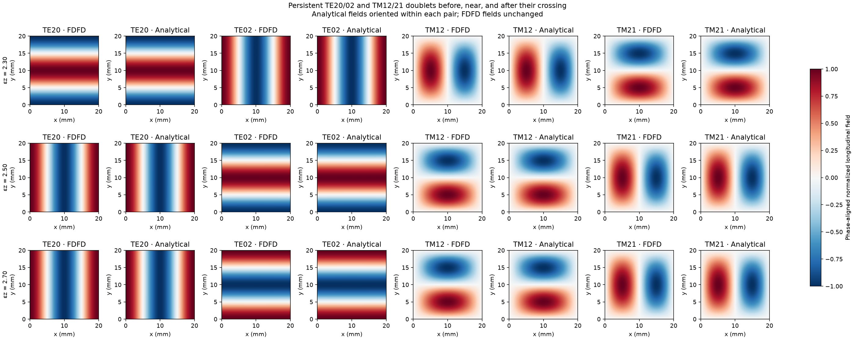
Equal-parity singlets can still represent rotated partners. Within one eligible longitudinal family, the axis-sensitive step compares variation along u and v and selects combinations with distinct directional scores. For example, it converts the square-guide combinations TE20 +/- TE02 into individual TE20 and TE02 fields. The same operation accepts hybrid E/H fields. Unresolved directional scores retain the established basis.
Axis selection can combine different rotation irreps. Each anchor therefore
stores the original irreducible_basis separately from the final source
transform. axis_sensitive records the selected blocks and scores;
longitudinal records family selection. A source-block symmetry label such
as A2+B2 describes the irreps contributing to that source field.
Each group is tested independently. If C4v decomposition fails, C2v is tried
when supported; if neither succeeds, the group retains its power-whitened
basis at its full dimension. A requested direction can then orient a complete
two-mode parent with independent electric moments.
Two transverse electric moments cannot fully orient a group larger than two.
Trials check span closure, continuity, mixed eigen-residuals,
reconstructed Maxwell residuals when available, positive full-group power,
and unit power within each retained block before
publishing any fields. SIBC ports additionally certify retained electric and
magnetic samples, complex boundary permittivities, and signed circulation
coefficients per retained dual area. Symmetric copper walls can therefore
use the same decomposition and axis selection; uncertified boundaries and
unsupported transverse solvers use the fallback. HDF5 symmetry_detection records detected
symmetries at each anchor, the applied choice per group, and rejected-trial
reasons; symmetry_subspaces stores successful decompositions.
Before accepting a selected basis, the complete power-wave measurement bank
must pass the modal coefficient solver’s precision budget for both electric
and magnetic Gram matrices, including coupling to modes outside the selected
group. Single precision allows a condition number of about 8.4e3;
double precision allows 1e10. The separate positive-power and symmetry
checks also apply. A rejected trial tries the next certified symmetry and
then retains the fallback basis if needed. Inspect the rejected-trial reasons
in symmetry_detection when the selected basis differs between precisions.
Neighboring fields continue the selected families and orientations across
frequency. The original tracking group remains available in
degenerate_groups; the selected source subspaces and their transformations
are stored in symmetry_subspaces in the HDF5 output.
Explicit mode_polarizations is applied after automatic subgroup selection.
The native symmetry basis passes mirror-parity checks before the requested
rotation. A diagonal polarized channel need not itself be a mirror eigenvector;
its two-dimensional span retains the certified symmetry. Final fields still
pass eigen-residual, Maxwell-residual, and measurement-conditioning checks.
symmetry_subspaces describes the certified basis before this rotation;
polarization_subspaces stores the pairwise rotations and requested directions.
The parent degenerate_groups transformations describe the final fields.
TE/TM and HE/EH conventions
TE modes have zero longitudinal electric field, \(E_w=0\); TM modes have zero longitudinal magnetic field, \(H_w=0\). Dielectric guides generally support hybrid modes, with both components nonzero. We use HE and EH for the conventional hybrid families. Their identification follows the vector fields and dispersion of a reference waveguide; the numerical longitudinal-content score alone does not assign an HE/EH name.
In an ideal circular dielectric guide, \(\mathrm{HE}_{mn}\) and \(\mathrm{EH}_{mn}\) use azimuthal order m and radial order n. The fundamental pair is \(\mathrm{HE}_{11}\). Sine/cosine angular partners belong to the same family and share the same indices. For rectangular or square dielectric cores, an HE-like or EH-like label refers to a stated reference-field convention; the circular angular/radial indices do not directly become transverse m/n indices. See the COMSOL vector hybrid-mode example and its HE/EH field comparisons.
The runtime retains stable branch labels B1, B2, and so on. These labels identify computed channels through frequency sweeps. Field plots may add a verified conventional name, while parity and symmetry labels describe the computed orientation.
Analytical validation
The validation gallery compares modal profiles and propagation constants for PEC rectangular, square, and cylindrical guides, an open dielectric cylinder, and persistent pairs crossing in an anisotropic square bore. Analytical fields check the computed channels and do not determine their runtime labels.
Warnings and inspection
A warning about the aperture is different from a failed mode solve or an uncertain mode identity. Use the following distinction when deciding what to change:
Result |
What happens |
What to inspect |
|---|---|---|
Suspected box mode or poor confinement |
A numerically valid, confidently tracked mode with forward power stays in use, with an accuracy warning. This warning alone does not remove anchors or change mode numbers. |
Check whether the field reaches the artificial edge. Enlarge the aperture and compare fields and S-parameters. |
Verification could not finish |
The result is unresolved, rather than proved good or bad. A usable primary profile is retained. |
Read the reason: surrounding geometry may be unavailable, refinement may be unsupported, or the extra-solve budget may be exhausted. |
Unsure which mode connects to the next anchor |
The tracker tries more candidates and intermediate frequencies. If still unresolved, it uses the automatic-anchor fallback or raises an error for explicit anchors. It does not interpolate across the gap. |
Inspect the fields on both sides of the uncertain interval and the anchor-selection message before trusting the broadband result. |
Failed numerical solution |
Fields that fail the equation checks, contain nonfinite values, or cannot be reconstructed or aligned reliably cannot supply a profile. |
Investigate the solve failure; enlarging a warning threshold does not repair unusable fields. |
A mode below cutoff is another case: decay along the guide does not make it a box mode. It may remain useful as a receiver reference, but a mode without usable forward power cannot be injected as a travelling power wave.
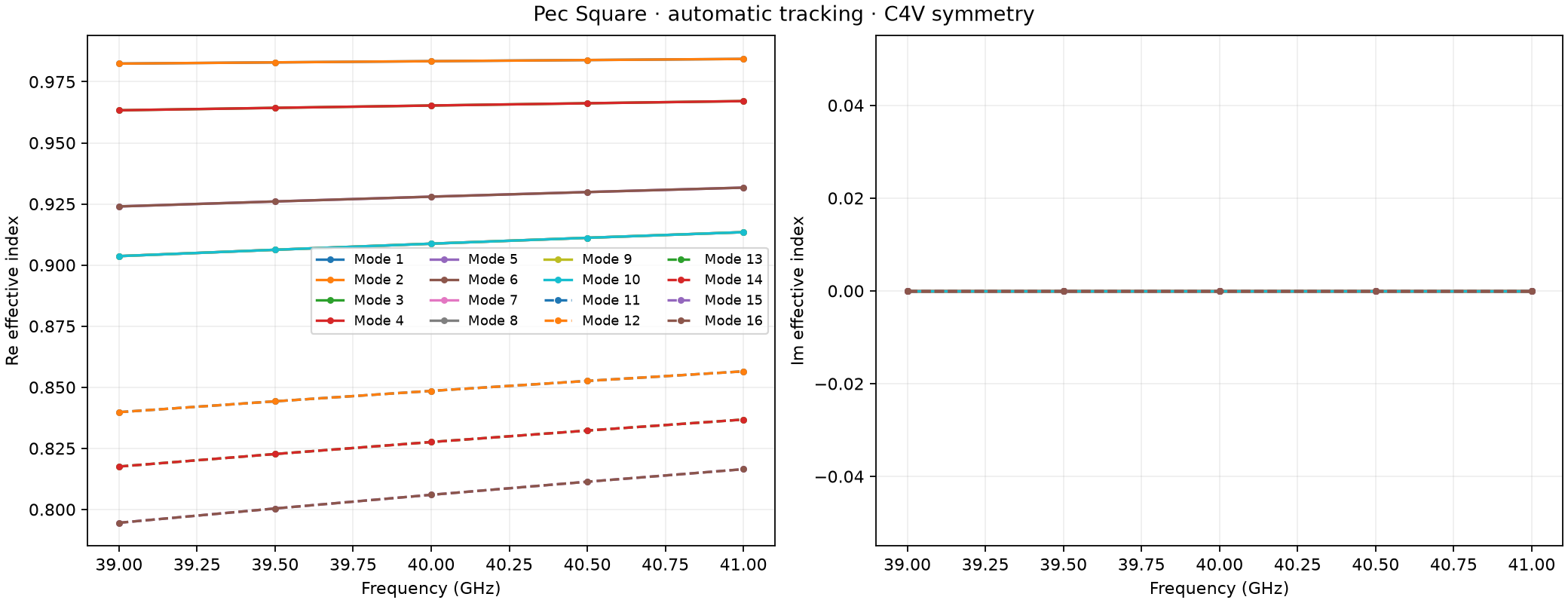
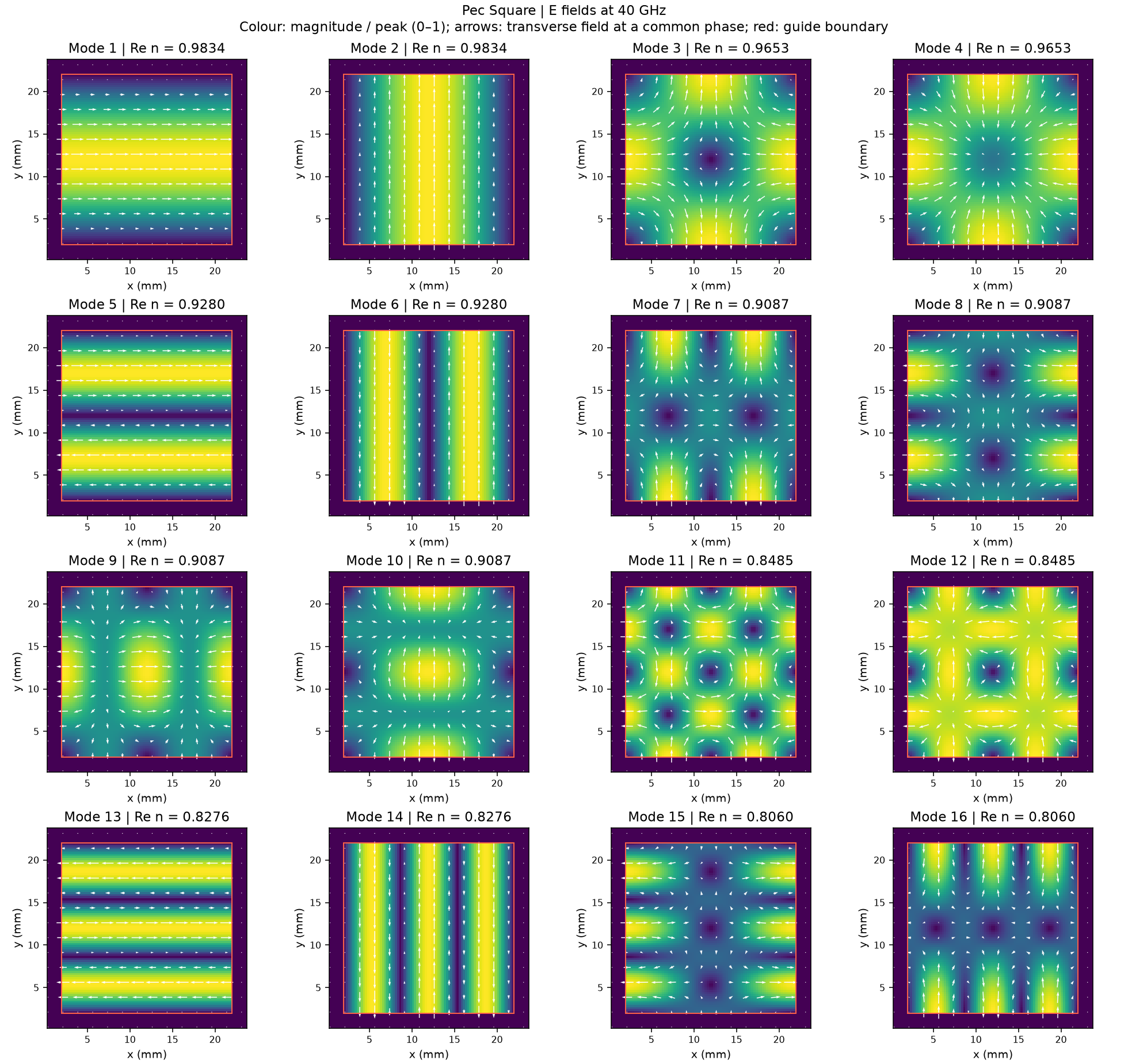
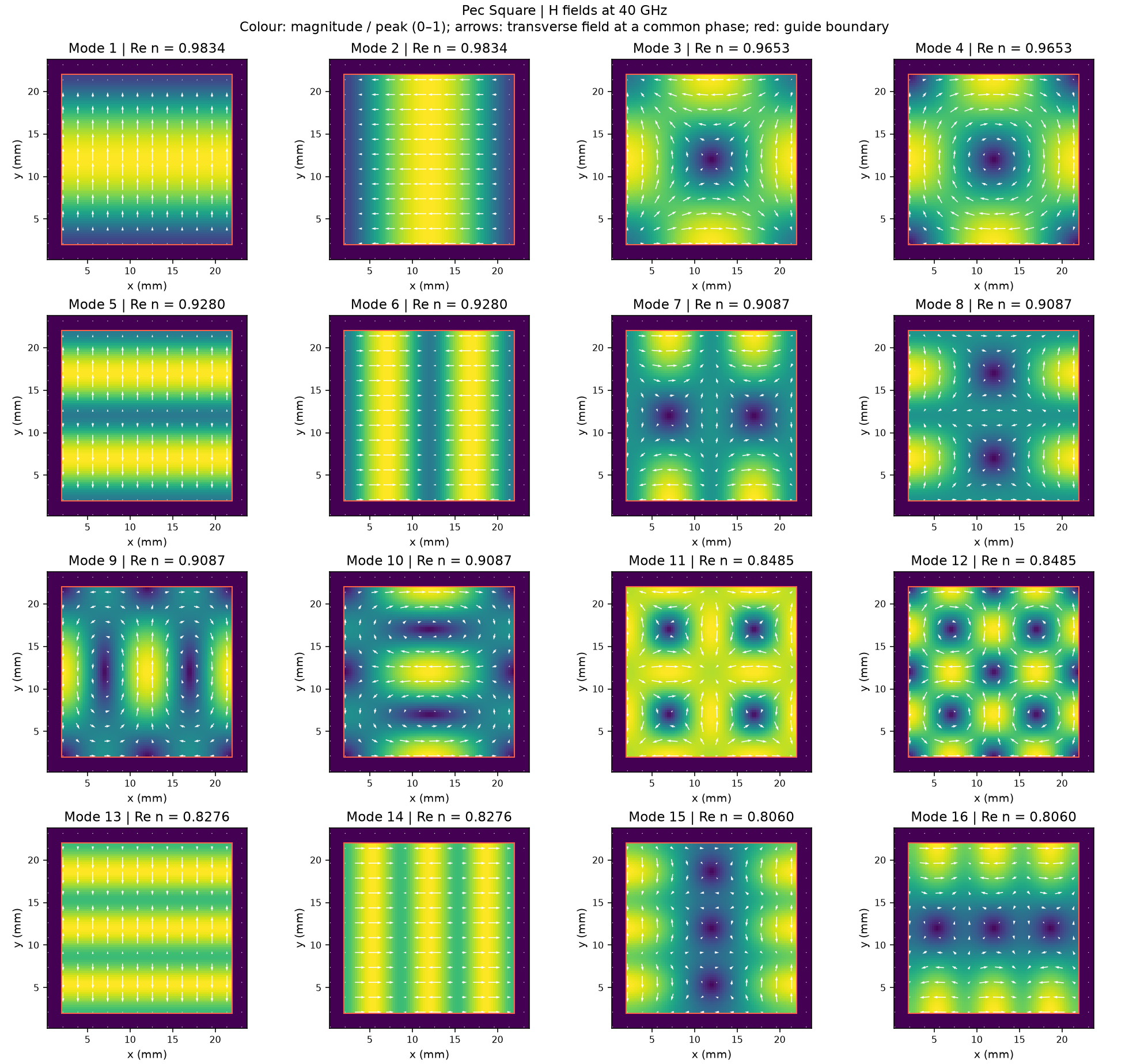
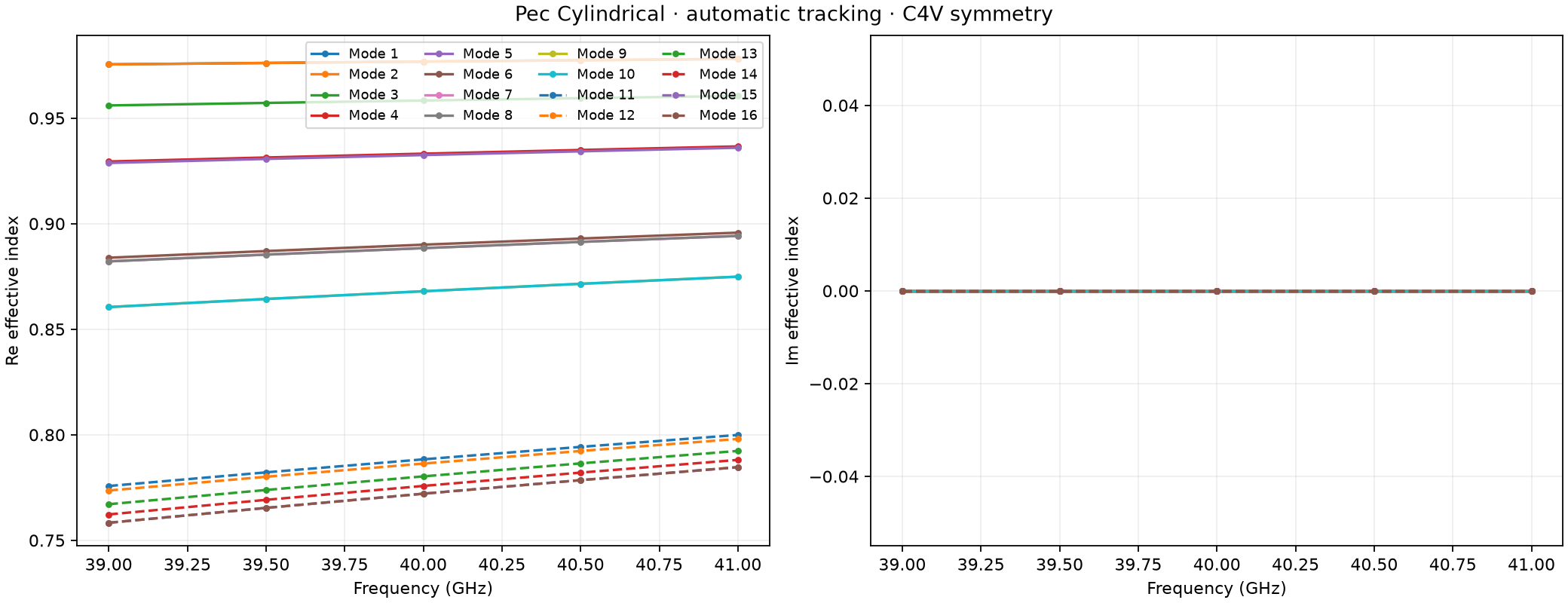
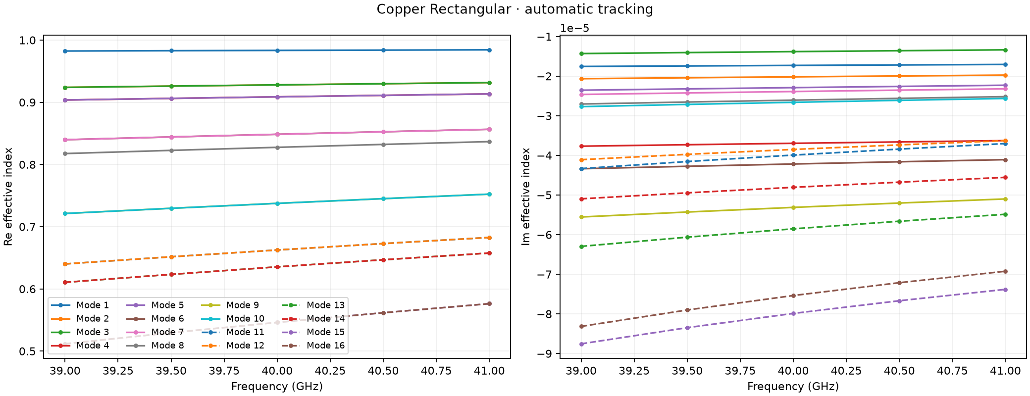
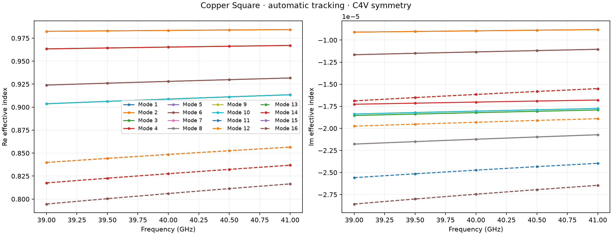
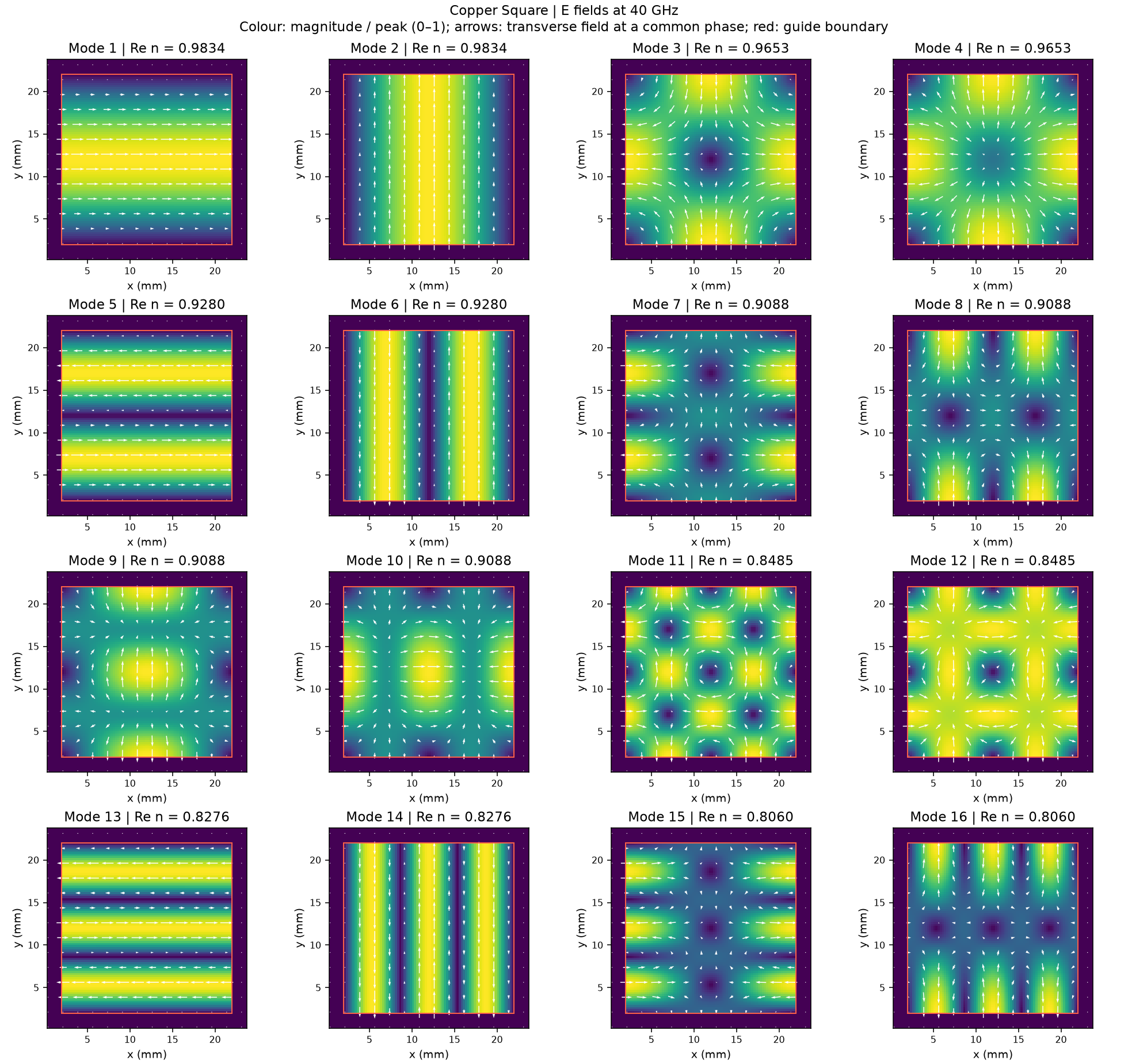
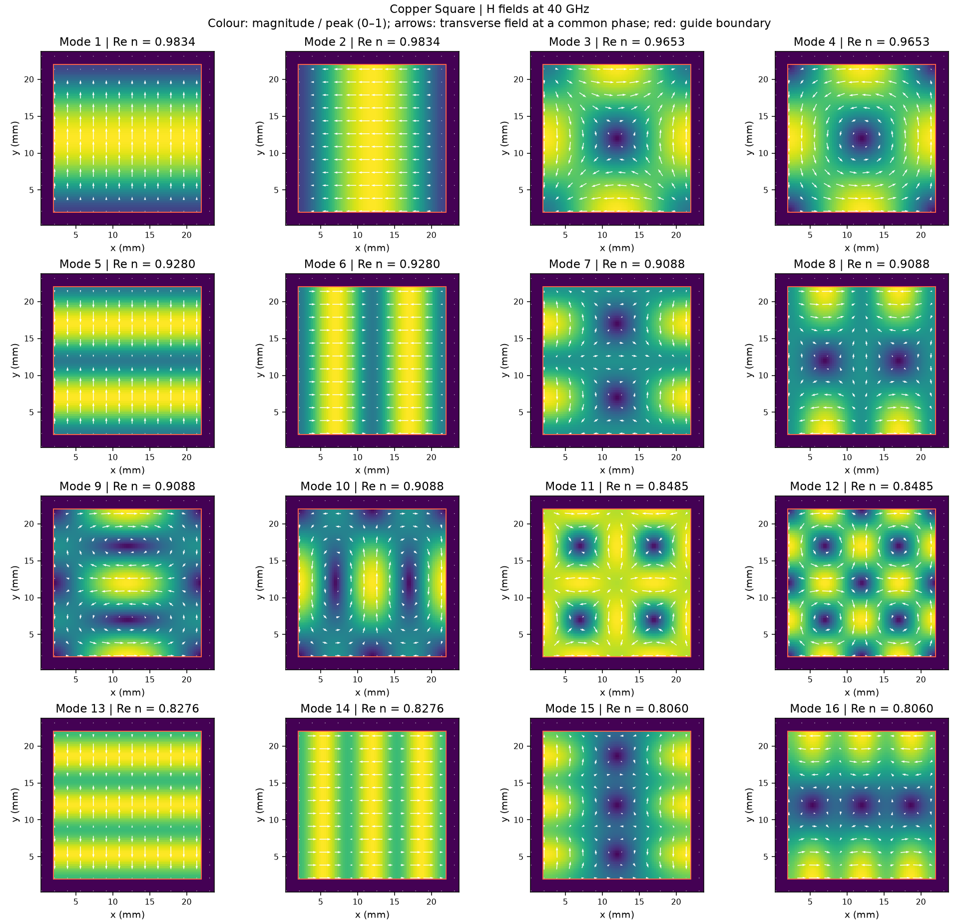
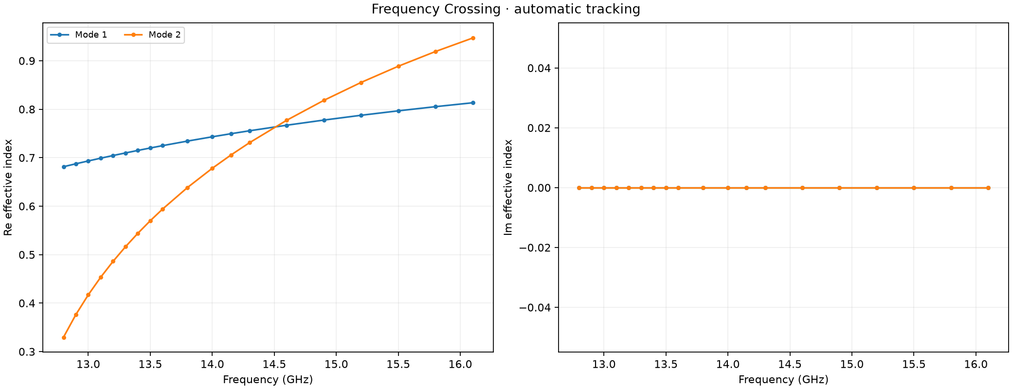
The figures place the dispersion curves, Re(n_eff) and -Im(n_eff),
above the E/H fields. The first shows how the phase propagation changes with
frequency; the second shows attenuation for the passive forward convention.
Diagnostic markers distinguish questionable profiles that remain in use
from missing or unusable profiles. A nonzero attenuation curve alone is not
evidence of a box mode.
For detailed inspection, the HDF5 mode_tracking group records which
solutions were matched, equation errors, verification evidence, and unresolved
intervals. Existing anchor and power validity masks keep their meanings.
The equations and exact decision rules are in
Eigenmode tracking theory.
Simulation examples
Start with the worked simulation below to follow the complete process: configure tracking at the source and receiving ports, inspect the modal bank, excite a tracked channel, run the simulation, and check the modal measurements. Afterwards, use the common-mode galleries to explore familiar field patterns and crossing behaviour. Independent analytical checks are in Eigenmode tracking: analytical validation.
Worked simulation: the circular TE11 pair
The complete model is
examples/features/eigenmode_ports/example_8_auto_degenerate_te11.
It constructs a straight circular PEC guide with a source port, a receiving
port, and a virtual-waveguide feed. Both ports use tracking="auto" and
request the two TE11 channels. The tracker detects their persistent pair
and selects reproducible default global x/y polarizations. A single shared
polarization direction can rotate those axes. Requesting only modes=(1,)
still solves its missing partner internally.
Configure the guide and ports. Define the 20–24 GHz eigenmode band, place matching source and receiving apertures, and set
tracking="auto"on both ports. Use the same mode request and polarization convention at each end. Explicit anchors cover the band and pulse spectral guards. The bore usesaveraging="y"to preserve shared PEC wall samples; see PEC wall construction and averaging.Inspect a geometry-only run. Check the dispersion and E/H profiles before excitation. The TE11 channels should have coincident propagation curves and stable orthogonal orientations. Inspect
mode_trackingdiagnostics for numerical validity and unresolved intervals. Resolve aperture or sampling problems before continuing.Choose the launched channel.
EigenmodeExcitation(port=1, mode=1,
waveform="auto")
launches the first tracked polarization. Changingmodeto 2 launches its partner. The virtual guide terminates the feed; the receiving end continues into the domain PML.Run the full simulation. Omit the geometry-only option and use the same port definitions. Repeat with the second launched mode to measure the other polarization.
Check the modal measurements. Plot co- and cross-polarized S11/S21 and the receiver traces. Interpret scattering results only where the output power-wave validity masks accept them. Confirm that channel identities remain consistent at both ports, then refine anchors, mesh, aperture, or terminations as needed for the intended accuracy.
Run these commands from the repository root in that order:
python examples/features/eigenmode_ports/example_8_auto_degenerate_te11/auto_degenerate_te11.py --geometry-only
python examples/features/eigenmode_ports/example_8_auto_degenerate_te11/auto_degenerate_te11.py --mode 1
python examples/features/eigenmode_ports/example_8_auto_degenerate_te11/plot_results.py --mode 1
python examples/features/eigenmode_ports/example_8_auto_degenerate_te11/auto_degenerate_te11.py --mode 2
python examples/features/eigenmode_ports/example_8_auto_degenerate_te11/plot_results.py --mode 2
plot_fields=True writes modal-profile figures in geometry-only and full
runs. The result plotter produces the modal S-parameter and receiver-trace
figures after each full run. This example uses verification="fast" for
inspection; when adapting the model, omit that setting or select "full"
for the additional convergence checks. In the recorded double-precision
CPU run, worst co-polarized S11 was about -62.9 dB for either polarization,
with co-polarized S21 near 0 dB.
Worked simulation: branch crossing in a square anisotropic guide
Example 9 under eigenmode_ports uses a 16 × 16 mm square PEC bore filled
with diag(2.25, 1, 1). The TE10 branch polarized along y and TE02 branch
polarized along x start as modes 3 and 4; their propagation curves cross
near 14.4 GHz on this mesh. These are higher-ranked channels rather than the two lowest
modes. Both ports request modes=(3, 4) and tracking="auto". Their
tracked labels remain stable as the raw eigenvalue ranks exchange.
Follow the same full process as the circular-pair example: inspect the geometry-only dispersion and modal fields, choose one tracked channel to launch, run the simulation, and inspect co- and cross-channel scattering with valid power-wave masks. Explicit anchors cover the 13.1–15.8 GHz band and its guards. Walls are built after the anisotropic fill to preserve the modal/FDTD boundary agreement, and sixteen-cell PMLs terminate both ends. An off-centre receiver samples both Ex and Ey; the TE02 field is zero at the bore centre.
python examples/features/eigenmode_ports/example_9_C2v_square_anisotropic_crossing/auto_mode_crossing.py --geometry-only
python examples/features/eigenmode_ports/example_9_C2v_square_anisotropic_crossing/auto_mode_crossing.py --mode 3
python examples/features/eigenmode_ports/example_9_C2v_square_anisotropic_crossing/plot_results.py --mode 3
python examples/features/eigenmode_ports/example_9_C2v_square_anisotropic_crossing/auto_mode_crossing.py --mode 4
python examples/features/eigenmode_ports/example_9_C2v_square_anisotropic_crossing/plot_results.py --mode 4
The result plots mark the tracked crossing and show the launched channel’s reflection and transmission alongside the interior probe polarization. This demonstrates automatic tracking during a driven simulation; the later crossing galleries inspect undriven modal banks.
Complete square-guide simulation
and result plotter.
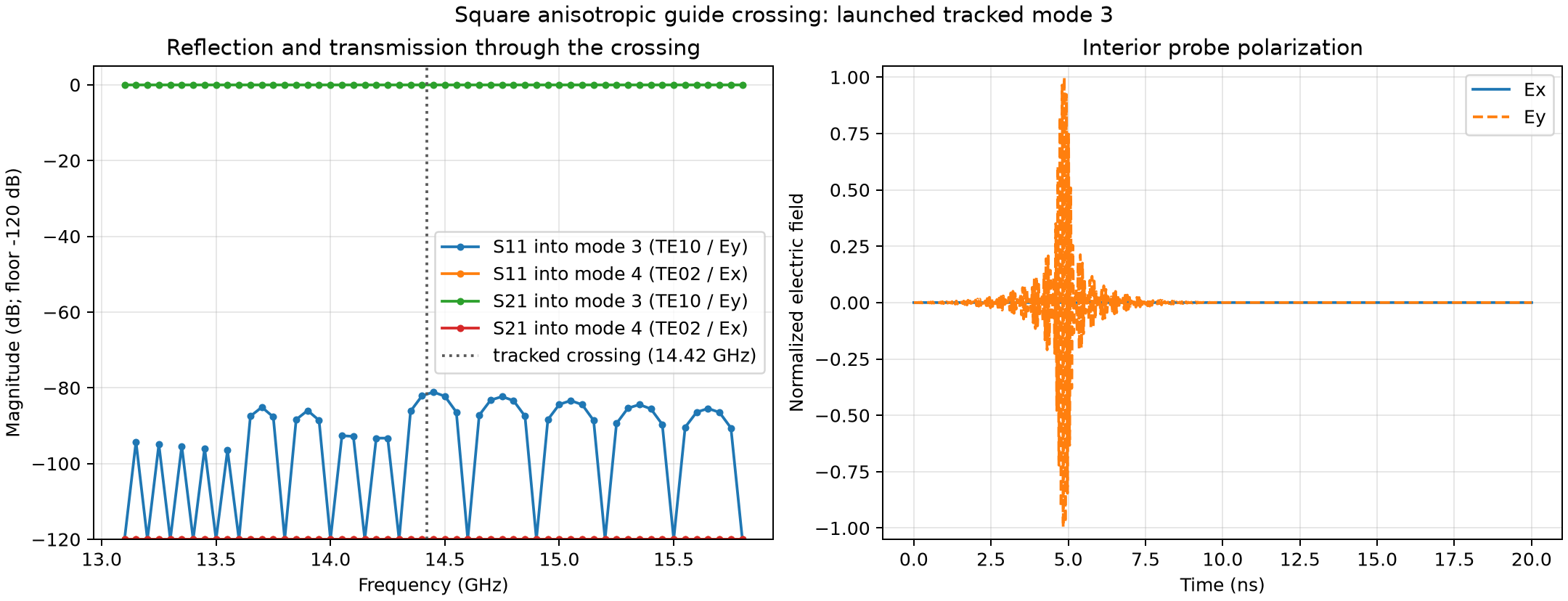
Fig. 18 Launching tracked mode 3: TE10 / Ey. The dotted line marks the crossing inferred from retained anchors. The receiver is at x = 10 mm, y = 6 mm.
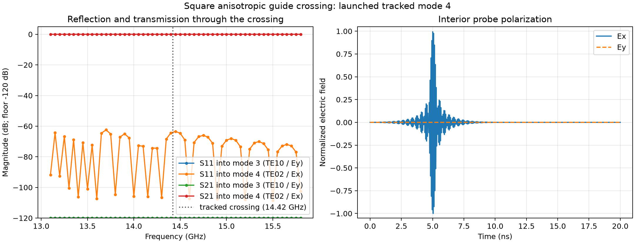
Fig. 19 Launching tracked mode 4: TE02 / Ex. Both full runs retain valid power-wave masks over the measurement band and have no unresolved tracking intervals.
The recorded double-precision CPU runs have worst co-channel S11 of
-81.1 dB and -62.4 dB for launched modes 3 and 4. The largest co-channel
S21 magnitude deviation from 0 dB is 0.000102 dB. These results concern the
represented mesh and port sampling; they do not establish convergence to
an exact continuum boundary. Recorded measurements.
Common-mode galleries
After following the simulation workflow, browse these galleries to recognize
tracked modes in common guides. Their scripts live under
examples/features/eigenmode_tracking and perform geometry-only runs.
They export native E/H fields and modal dispersion; they do not excite a
port or produce scattering measurements. Gallery numbers match the numbered
script folders, which are separate from the driven eigenmode_ports
tutorials above.
Choose a geometry and material
Gallery |
Guide |
Material |
|---|---|---|
C2v rectangular, 20 × 10 mm |
PEC |
|
C4v square, 20 × 20 mm |
PEC |
|
Cylindrical, radius 10 mm |
PEC |
|
C2v rectangular, 20 × 10 mm |
Copper |
|
C4v square, 20 × 20 mm |
Copper |
|
Cylindrical, radius 10 mm |
Copper |
|
Rectangular core, 20 × 10 mm |
εr = 4 in air |
|
Square core, 20 × 20 mm |
εr = 4 in air |
|
Cylindrical core, radius 10 mm |
εr = 4 in air |
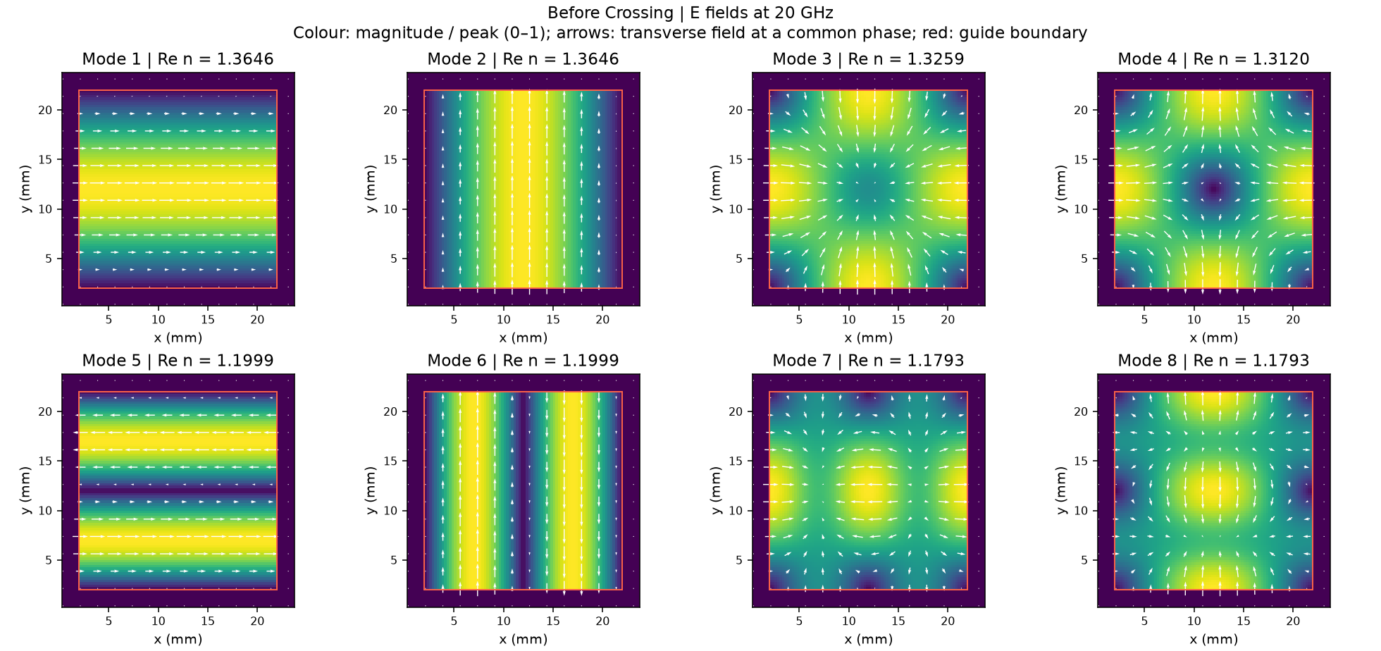
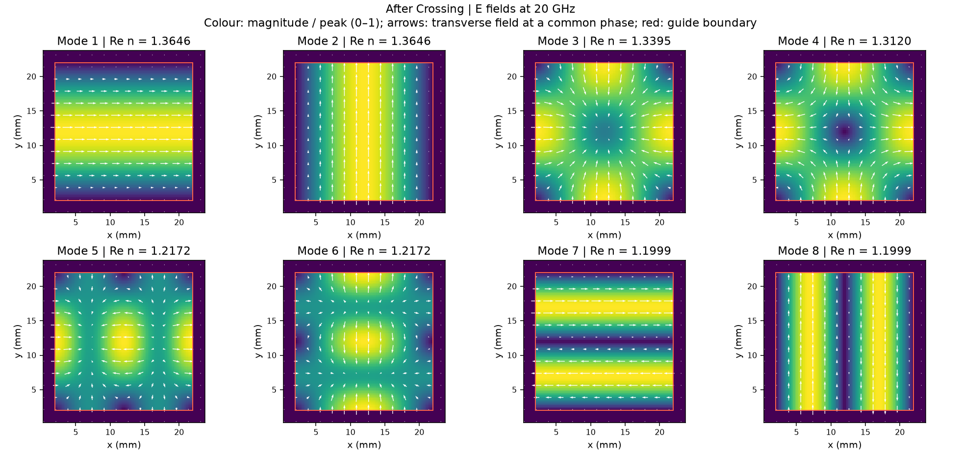
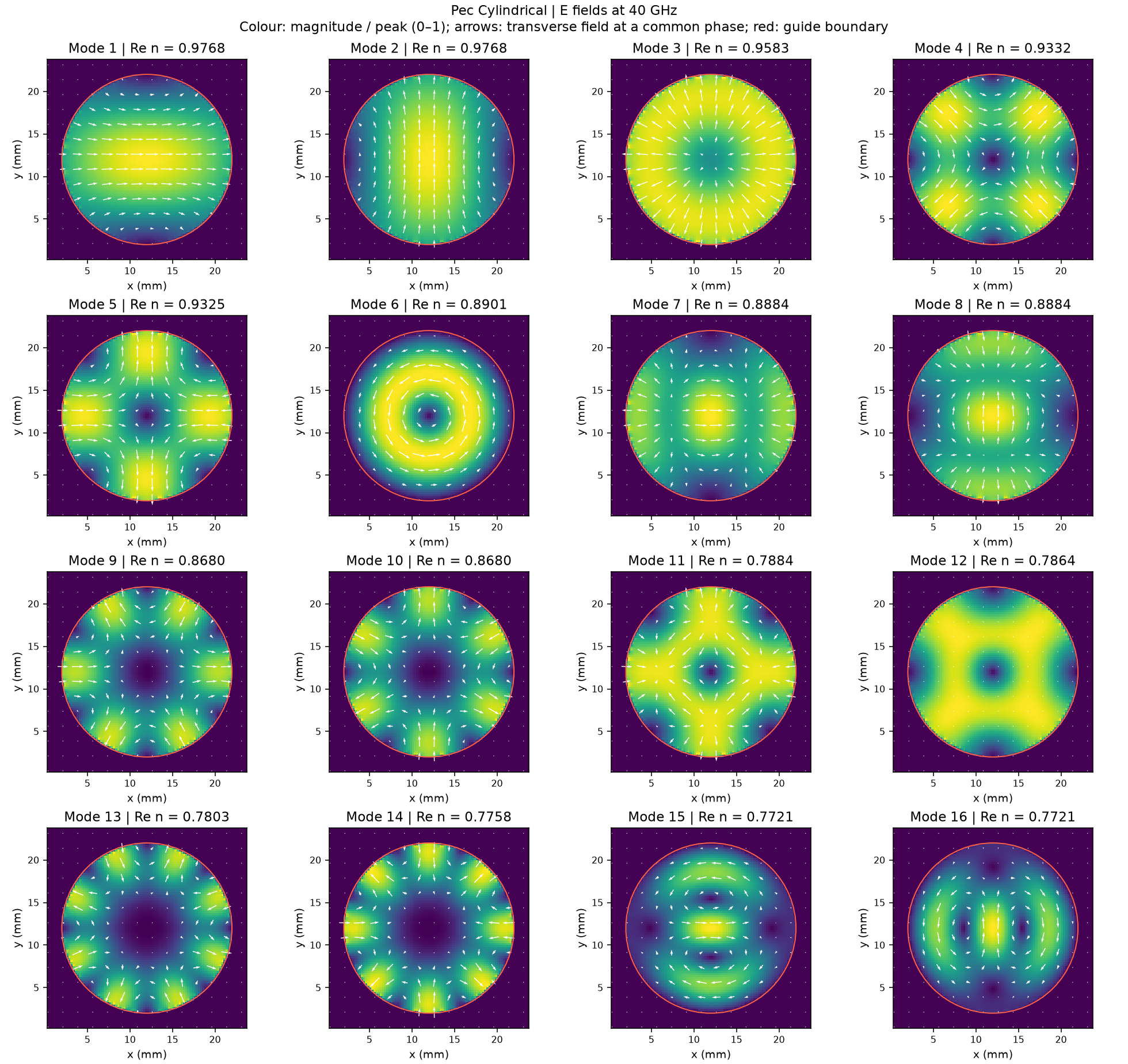
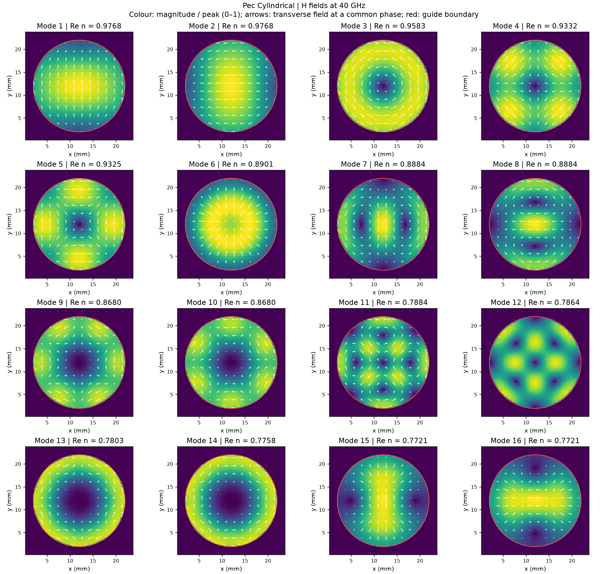
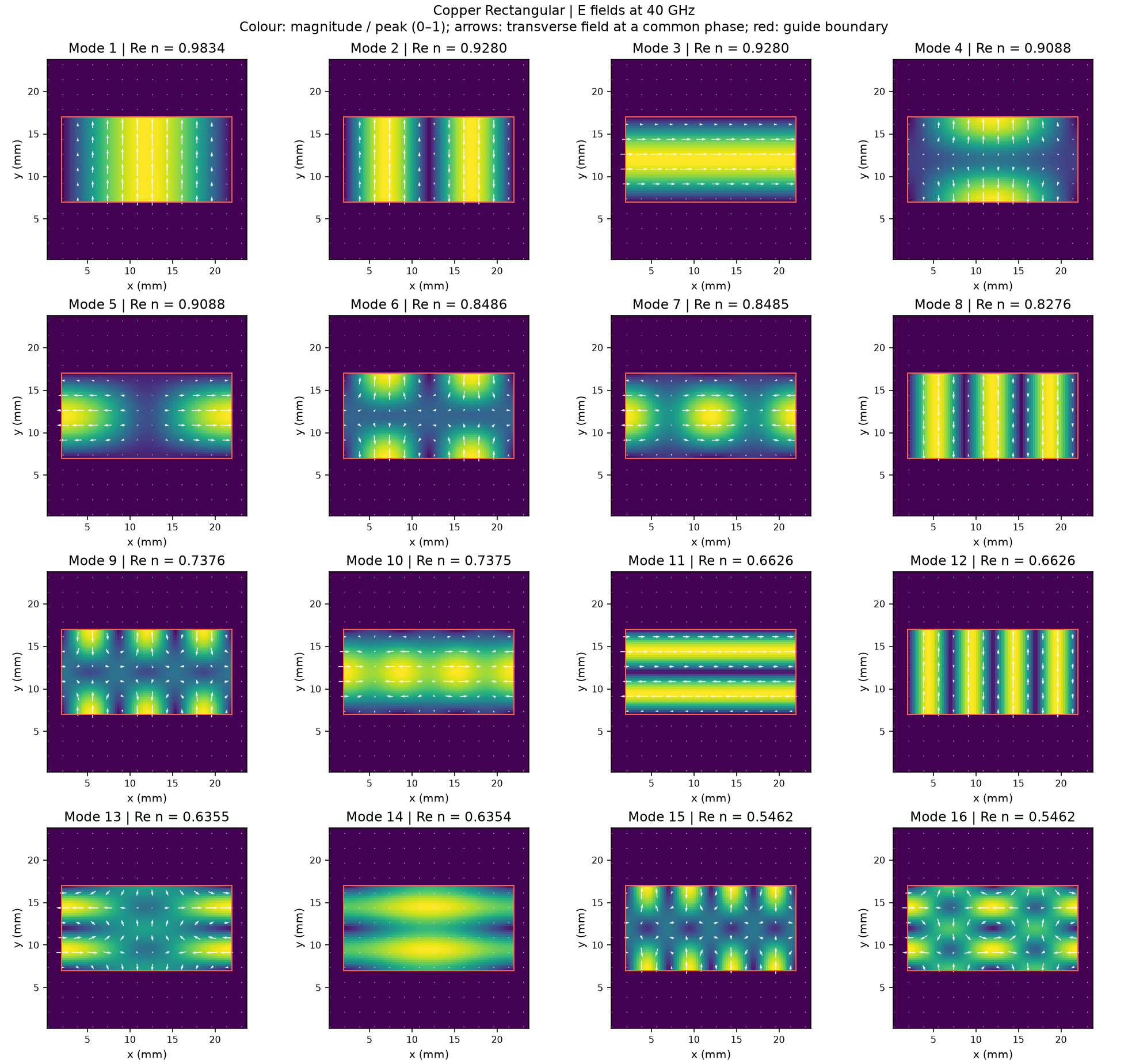
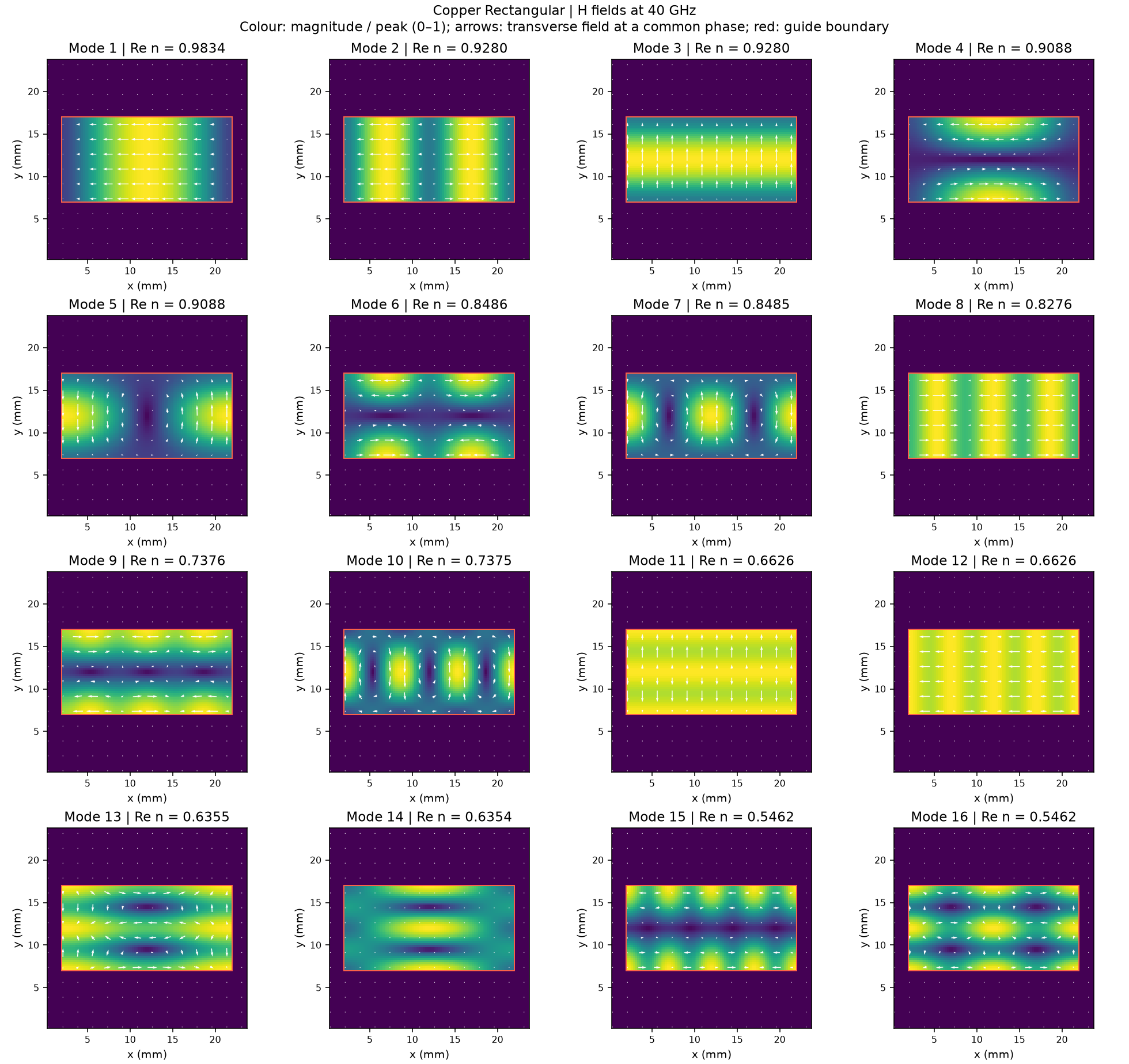
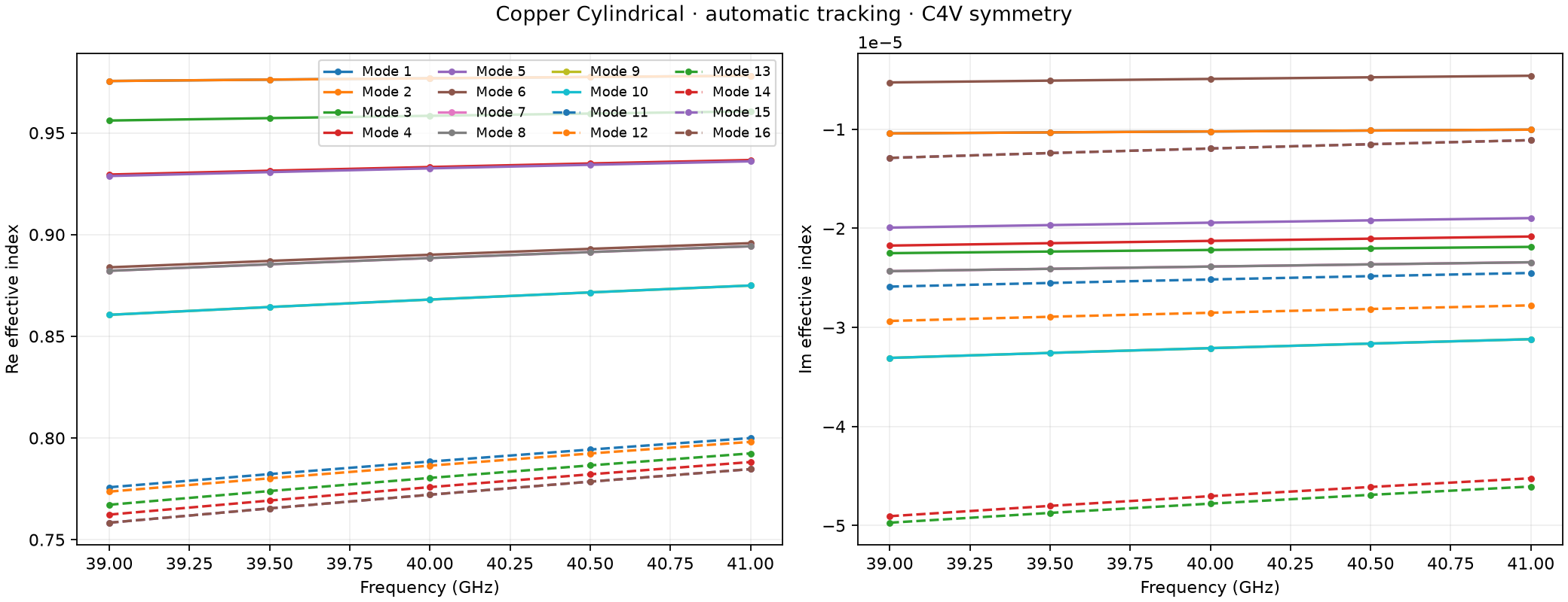
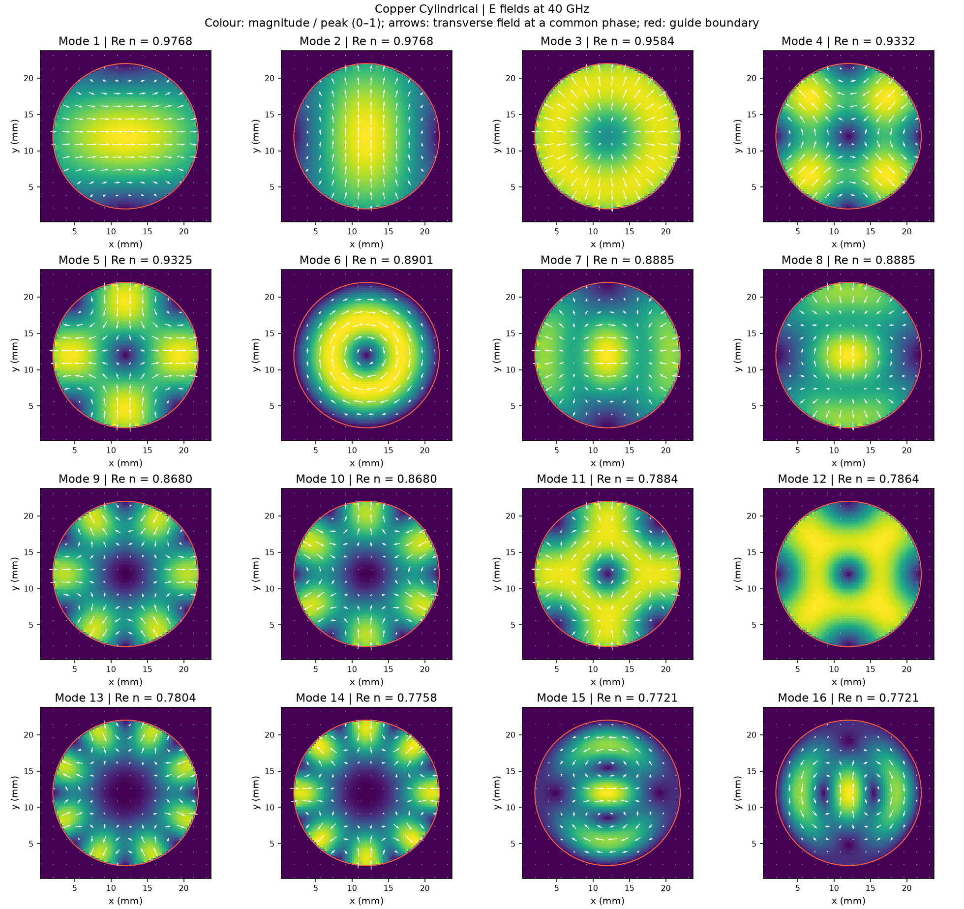
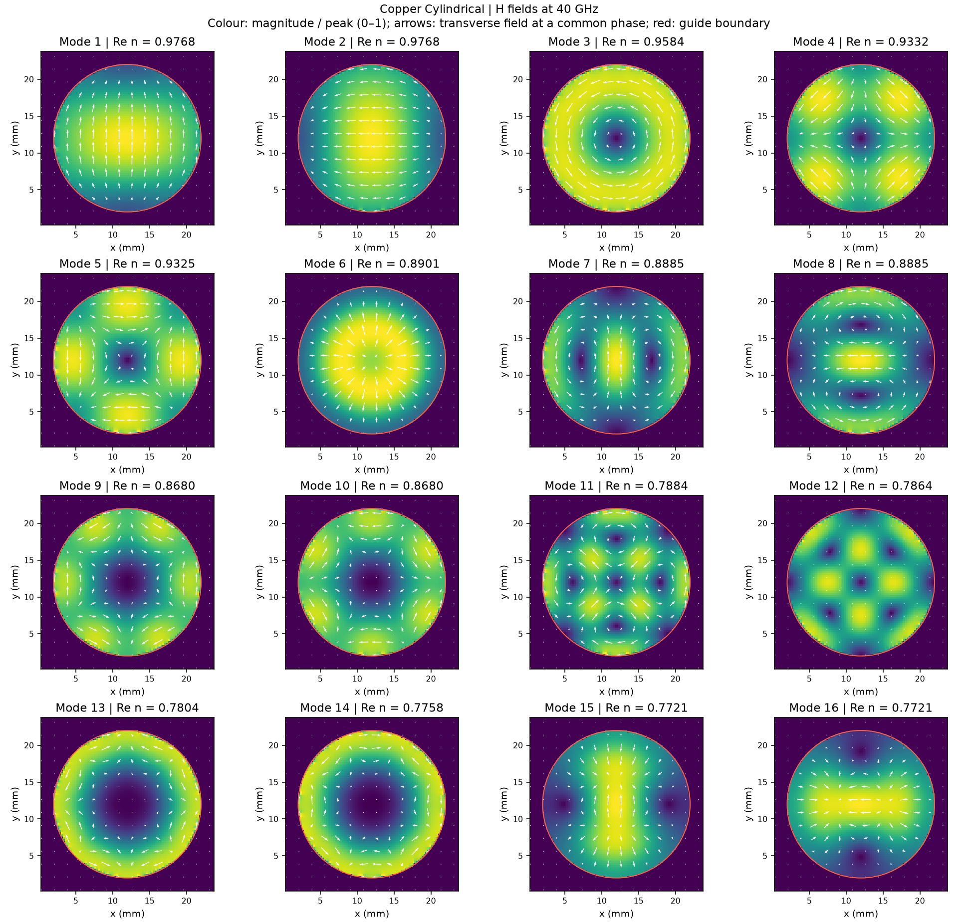
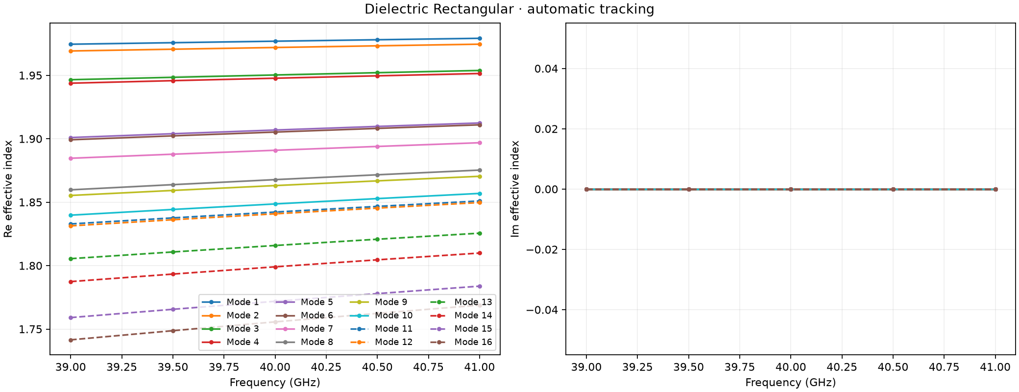
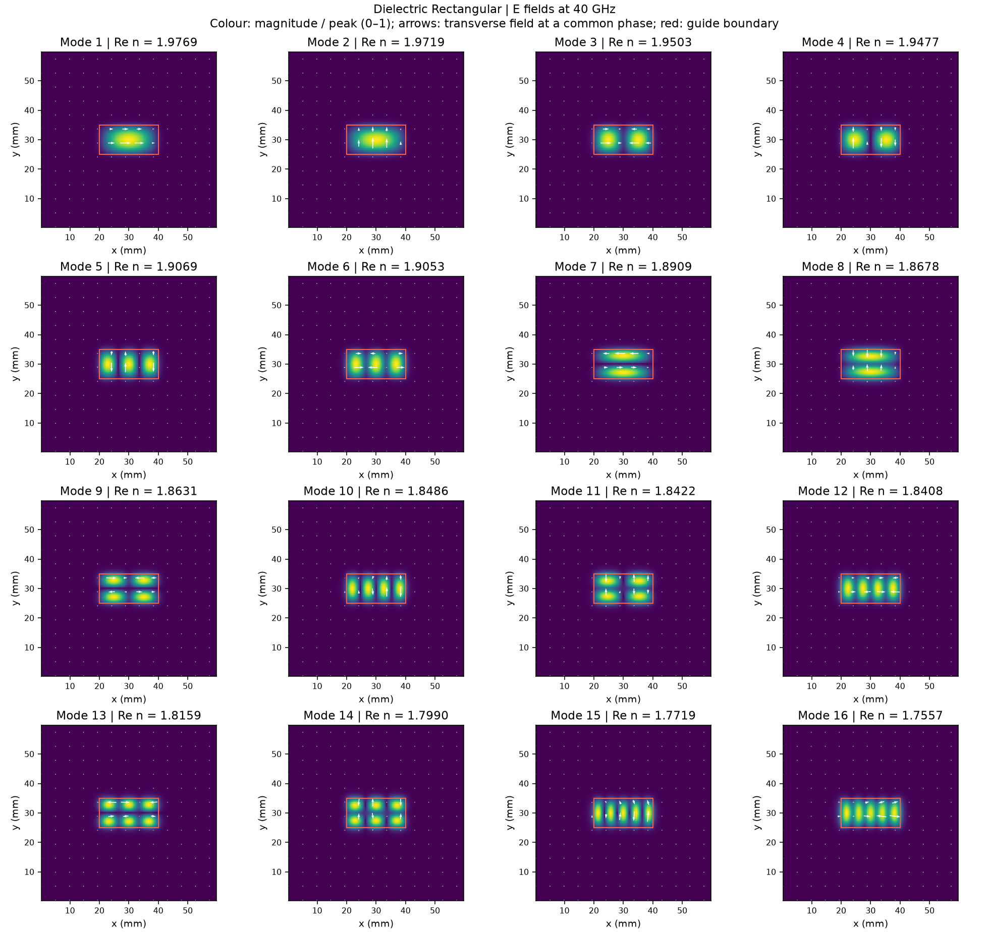
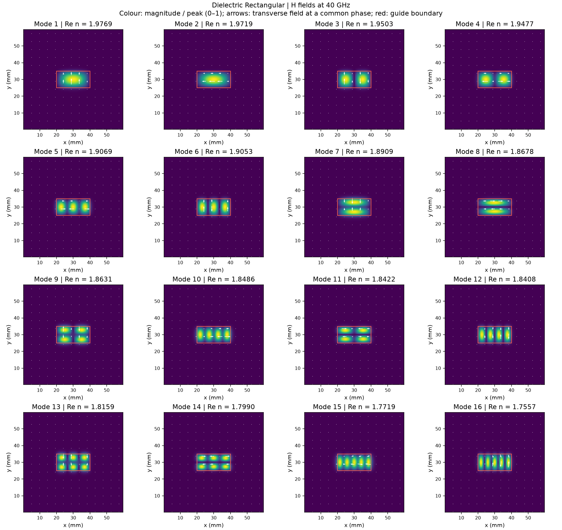
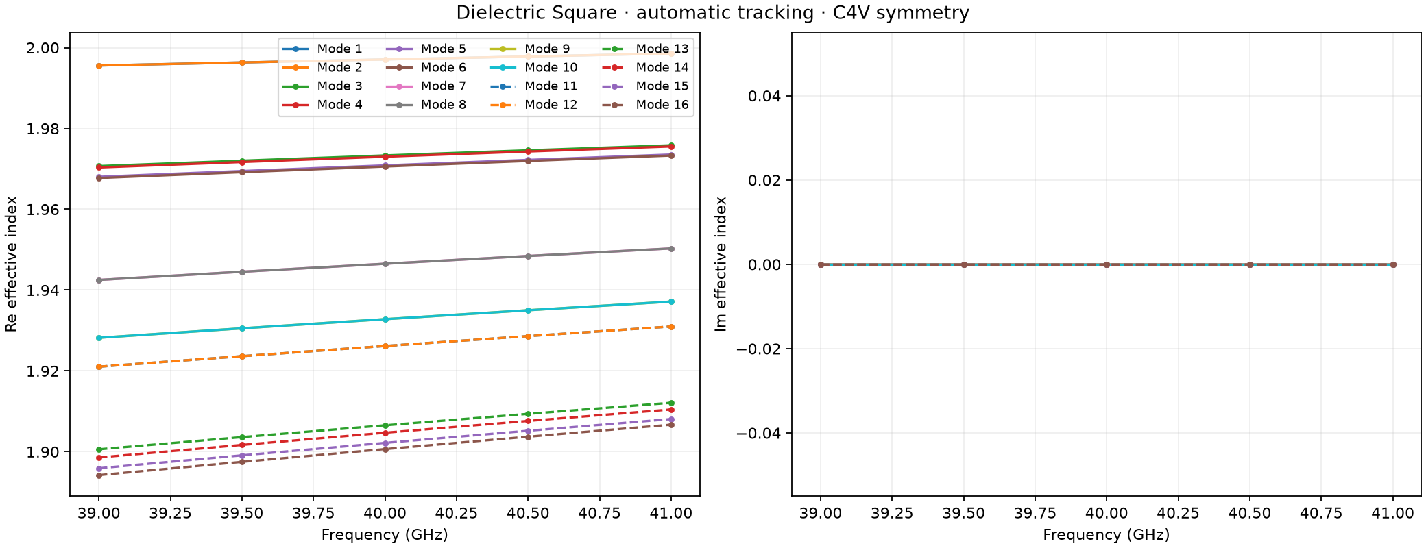
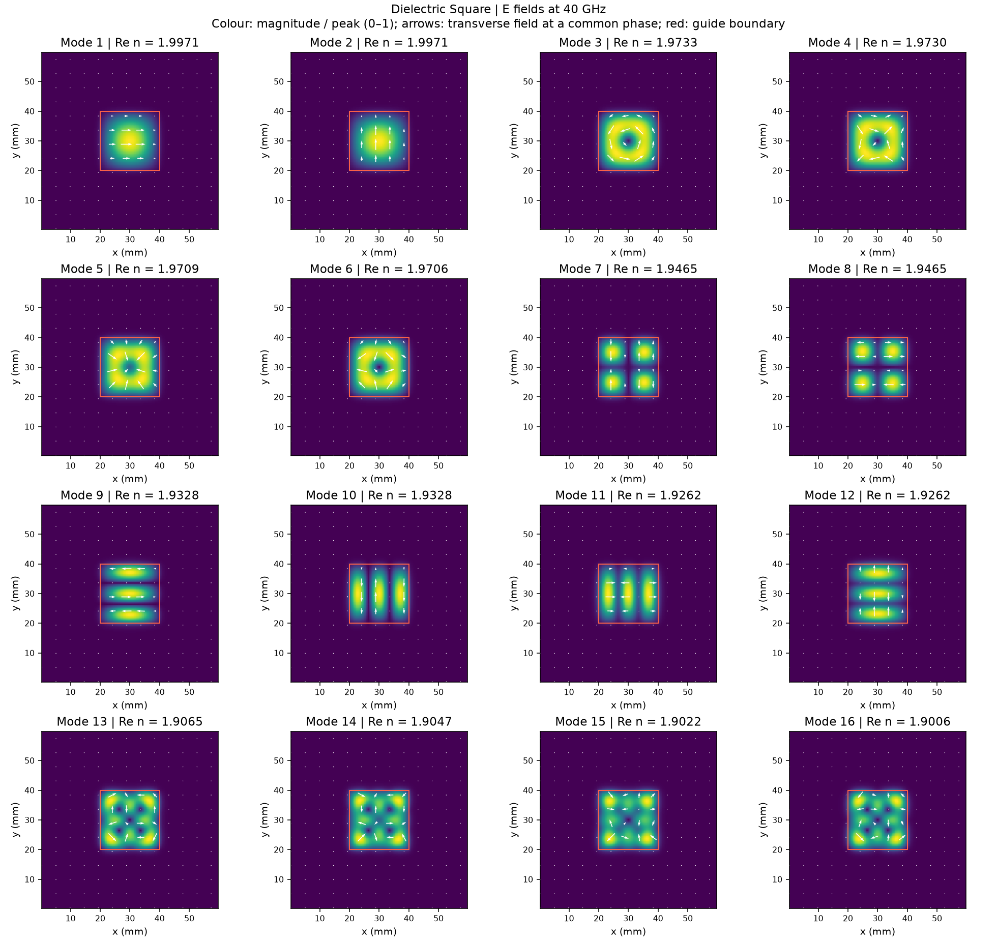
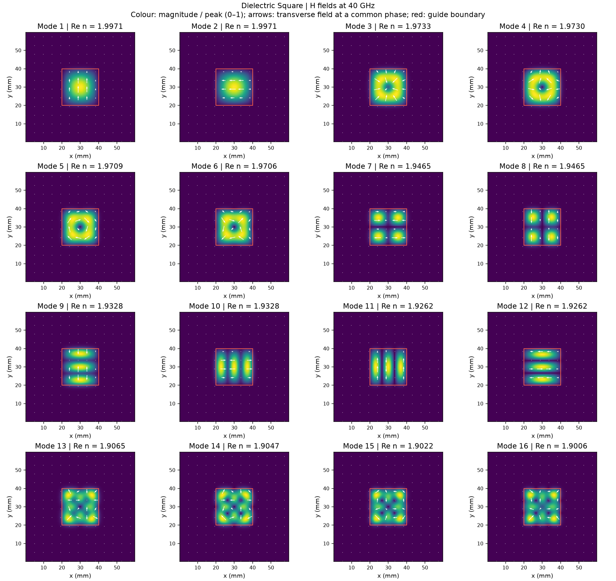
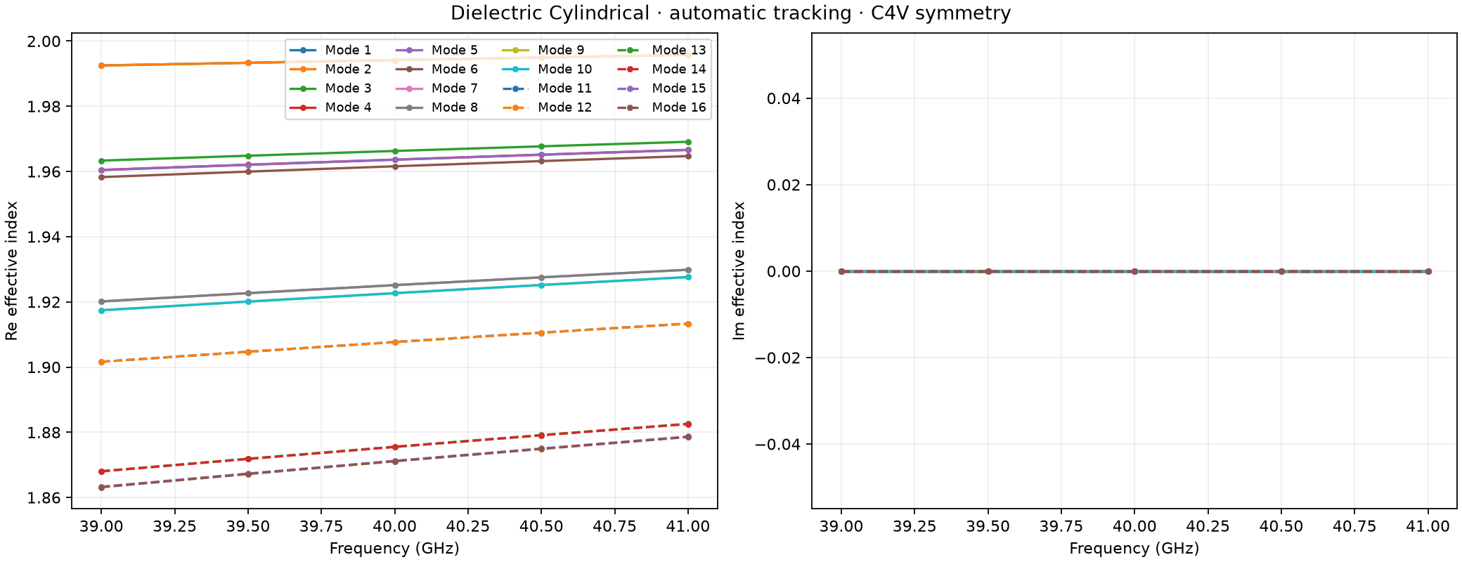
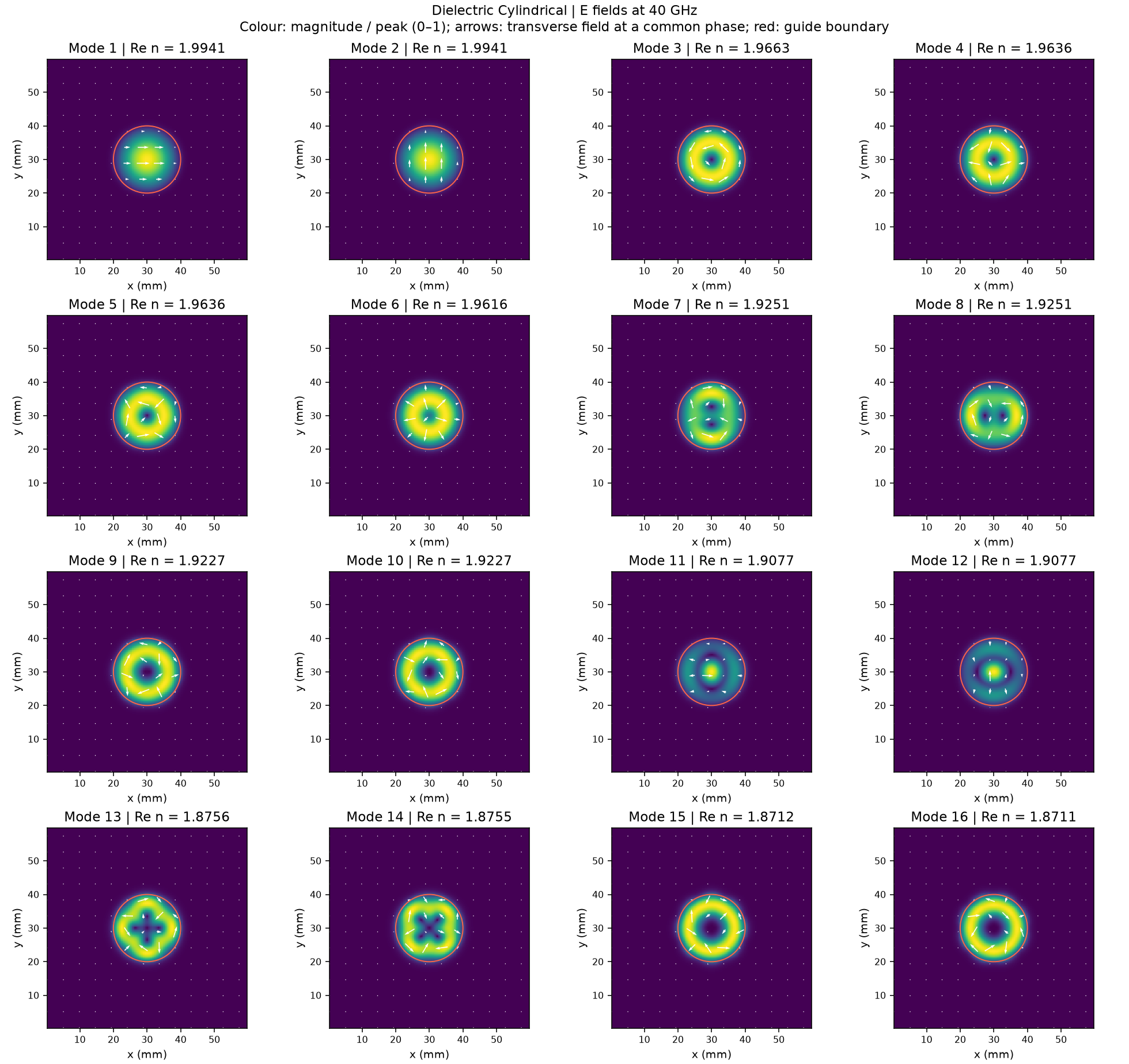
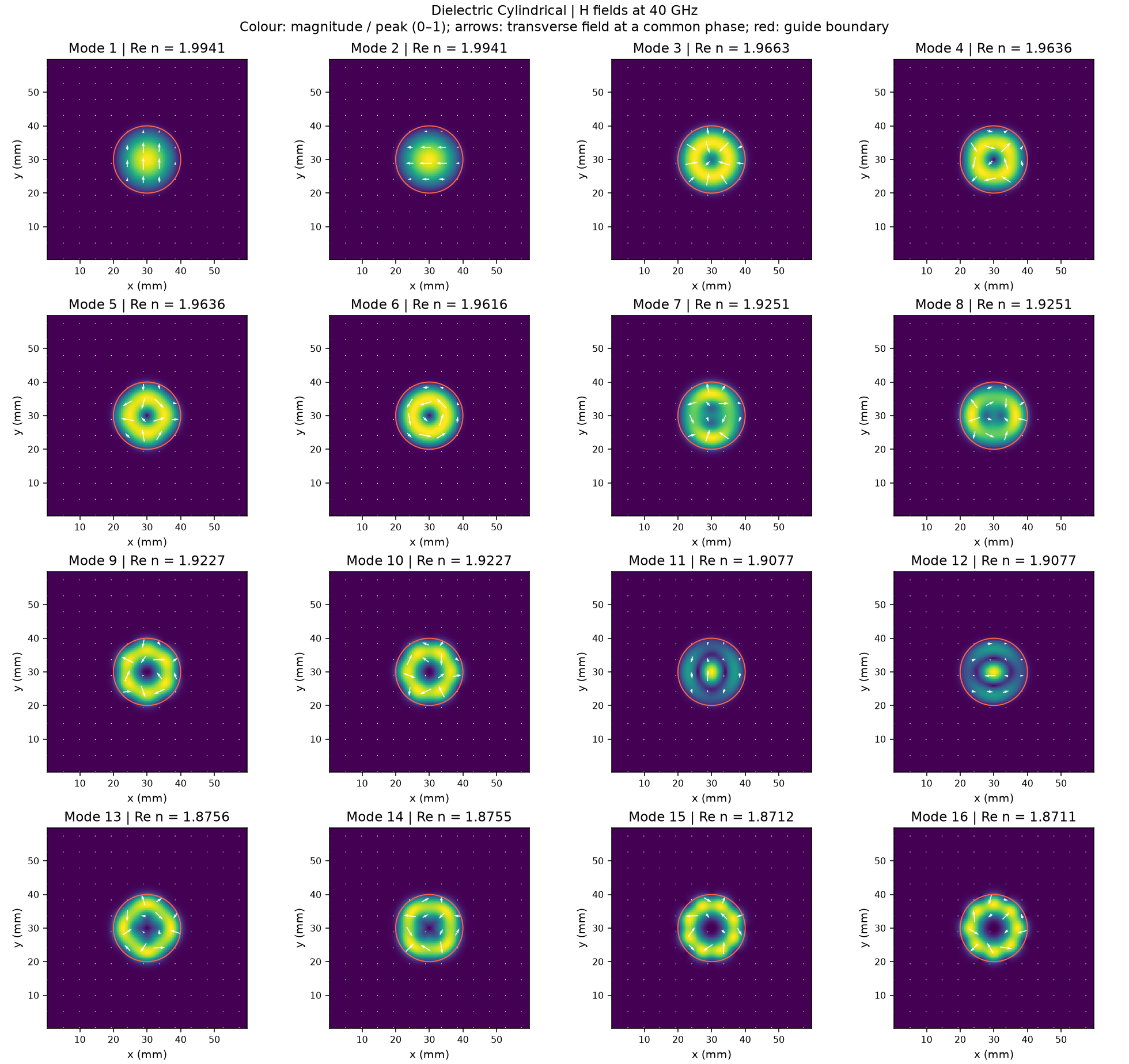
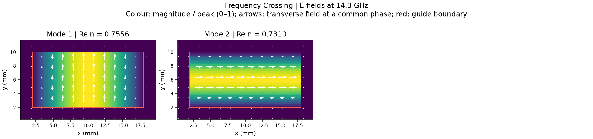
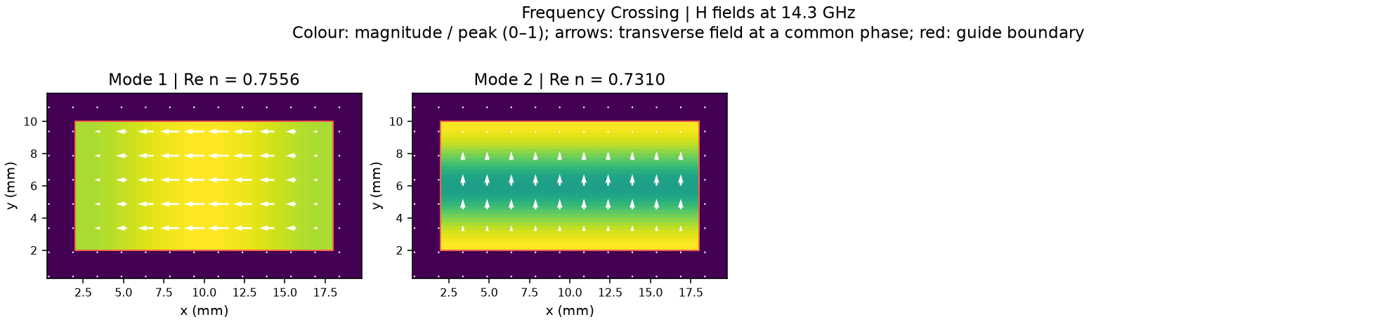
Each common-guide gallery shows sixteen channels over 39–41 GHz, with real/imaginary effective-index curves and E/H fields at the middle anchor. Colour gives field magnitude normalized per mode; arrows show transverse fields at a common phase. The default spacing is 0.25 mm. Copper uses the conductivity surface-impedance preset with an ADE fit over 1–120 GHz. Dielectric apertures have distant artificial PEC rims, and cylindrical boundaries are staircased. Detected symmetry labels describe that sampled problem.
To regenerate a gallery, run its script from the repository root, for example:
python examples/features/eigenmode_tracking/example_1_C2v_rectangular_PEC/tracked_modes.py
--spacing-mm changes the mesh, --modes changes the requested channel
count, --verification full adds convergence checks, and --output
selects a fresh result directory. Recorded galleries are separate from new
outputs. Analytical field and propagation-constant comparisons remain in
Eigenmode tracking: analytical validation.
Recorded common modes
Gallery 1: PEC rectangular tracked modes
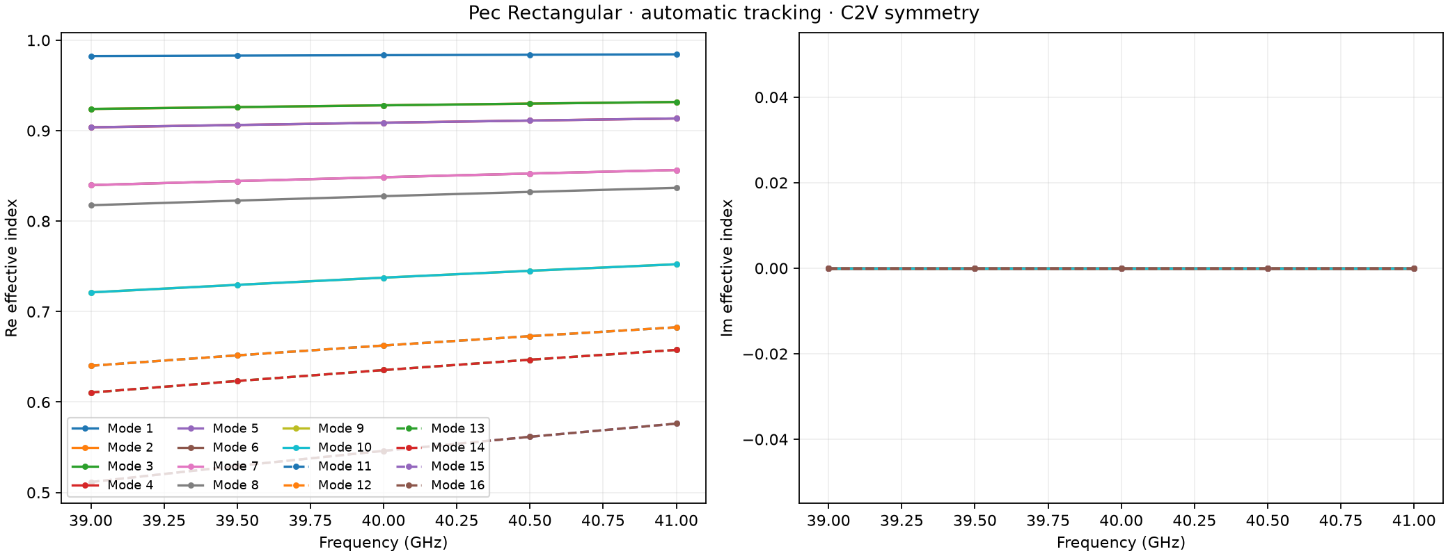
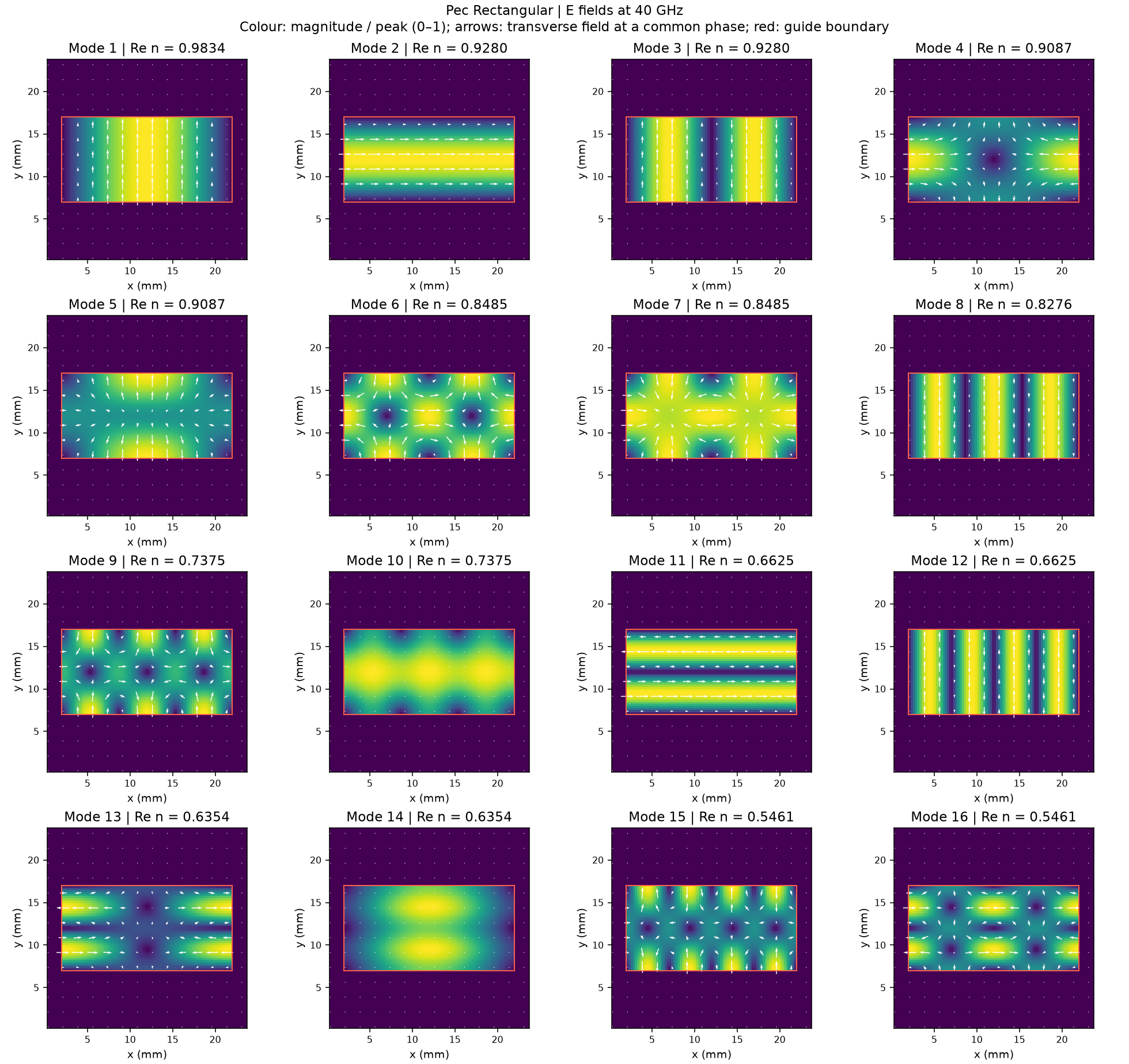
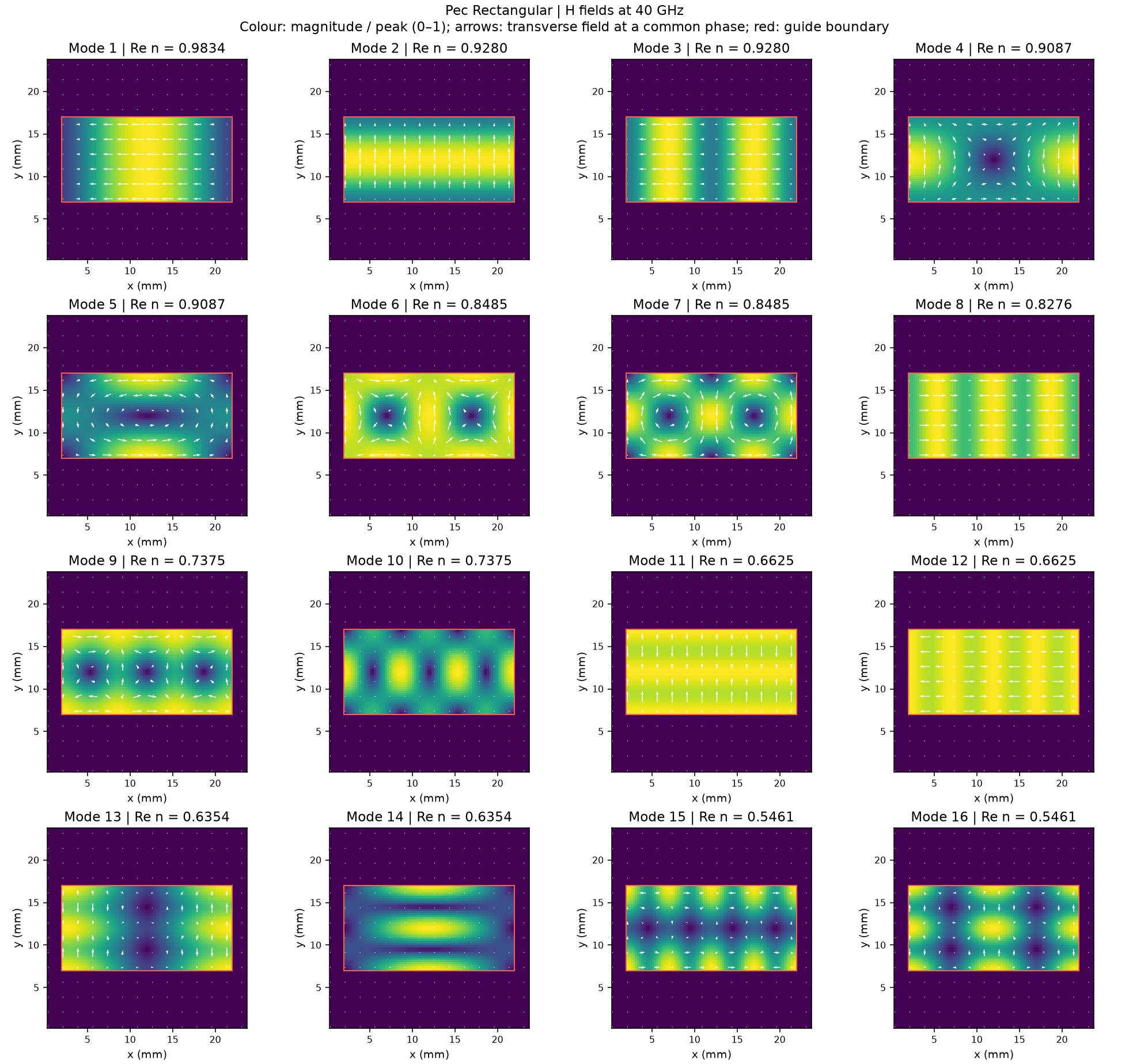
Gallery 2: PEC square tracked modes
Gallery 3: PEC cylindrical tracked modes
Gallery 4: COPPER rectangular tracked modes
Gallery 5: COPPER square tracked modes
Gallery 6: COPPER cylindrical tracked modes
Gallery 7: DIELECTRIC rectangular tracked modes
Gallery 8: DIELECTRIC square tracked modes
Gallery 9: DIELECTRIC cylindrical tracked modes
Crossing-mode galleries
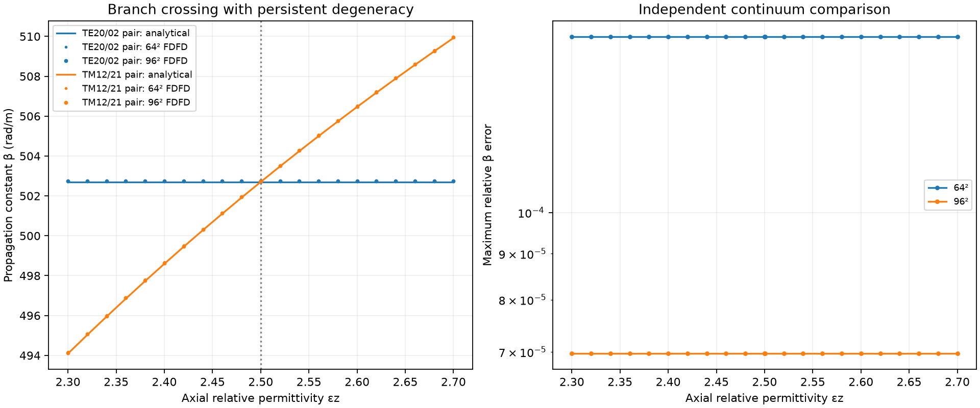
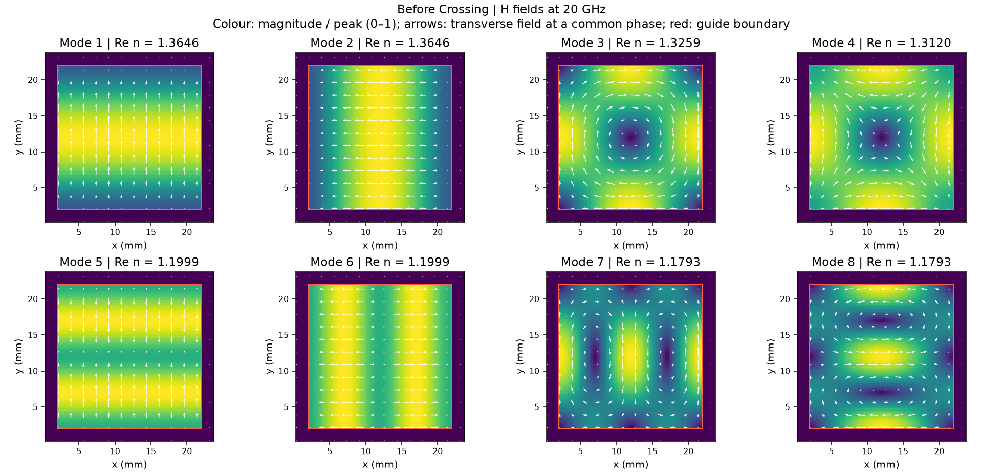
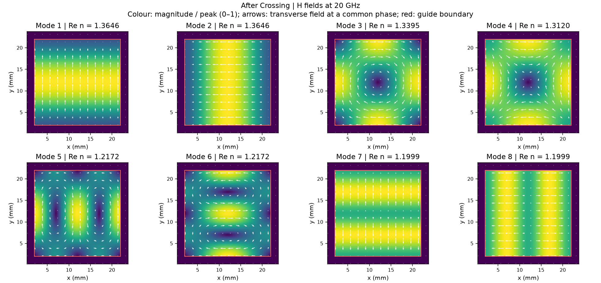
Gallery 10 follows two polarized branches crossing in frequency in an anisotropic rectangular PEC bore. Gallery 11 shows two persistent square- guide doublets crossing as axial permittivity changes at fixed 20 GHz. These focused cases use two and eight channels. Gallery 11 combines geometry-only native port snapshots with an undriven material-parameter FDFD sweep and analytical comparisons. At the exact numerical coincidence, all four input modes are deliberately mixed, and tracking recovers the two persistent pairs.
Regenerate them with:
python examples/features/eigenmode_tracking/example_10_anisotropic_frequency_crossing/tracked_modes.py
python examples/features/eigenmode_tracking/example_11_C4v_square_persistent_pair_crossing/tracked_modes.py
Gallery 10: Two polarized branches crossing in frequency
Gallery 11: Persistent doublets crossing in a square guide