Toolboxes is a sub-package where useful Python modules contributed by users are stored.

GPR Antenna Models

Information

Optional optimisation keyword names are checked. Unknown names raise TypeError instead of being ignored, even if their value is None or zero. Supply the documented parameter set for the selected antenna.

The package features models of antennas similar to commercial GPR antennas. The following antenna models are included:

Manufacturer/Model	Dimensions	Resolution(s)	Author/Contact	Attribution/Cite
GSSI 1.5GHz (Model 5100)	170x108x45mm	1, 2mm	Craig Warren (craig.warren@northumbria.ac.uk), Northumbria University, UK	1
GSSI 2GHz palm antenna	86x86x68mm	1mm	Ourania Patsia, Antonios Giannopoulos, and Iraklis Giannakis, The University of Edinburgh, UK	3
MALA 1.2GHz	184x109x46mm	1, 2mm	Craig Warren (craig.warren@northumbria.ac.uk), Northumbria University, UK	—
GSSI 400MHz	300x300x170mm	2mm	Sam Stadler (sam.stadler@leibniz-liag.de), Leibniz Institute for Applied Geophysics, Germany	2

License: Creative Commons Attribution-ShareAlike 4.0 International License

Attributions/citations:

1. Giannakis, I., Giannopoulos, A., & Warren, C. (2019). Realistic FDTD GPR antenna models optimised using a novel linear/non-linear Full Waveform Inversion. IEEE Transactions on Geoscience and Remote Sensing, 57(3), 1768-1778. (https://doi.org/10.1109/TGRS.2018.2869027)

2. Stadler, S., & Igel, J. (2022). Developing realistic FDTD GPR antenna surrogates by means of particle swarm optimization. IEEE Transactions on Antennas and Propagation, 70(6), 4259-4272. (https://doi.org/10.1109/TAP.2022.3142335)

3. Patsia, O., Giannopoulos, A., & Giannakis, I. (2024). Developing a realistic numerical equivalent of a GPR antenna transducer using global optimizers. Near Surface Geophysics, 22(2), 140-151. (https://doi.org/10.1002/nsg.12280)

Package contents

• GSSI.py is a module containing models of antennas similar to those manufactured by Geophysical Survey Systems, Inc. (GSSI).

• MALA.py is a module containing models of antennas similar to those manufactured by MALA Geoscience.

Descriptions of how the models were created can be found in the aforementioned attributions.

GSSI 2 GHz receiver-port update

antenna_like_GSSI_2000 now uses a zero-amplitude voltage source with the original 200008.0107 Ohm receiver resistance. Its rigid gap retains er=1.056; only the resistance has moved from material conductivity to the source, so the original loading and gssi2000_rxbowtie Ey output are preserved. The automatic voltage-source ports now have explicit IDs gssi2000_tx and gssi2000_rx (update references to the former automatic Tx portN). Receiver voltage is saved in /ports/gssi2000_rx/Vtotal with its own half-step time axis. Zero amplitude does not mean zero resistance or a clamp.

Use the driven Tx port for its input impedance and S11. The passive receiver’s generator is zero, so its own input S11/impedance cannot be inferred from this run; drive Rx separately with Tx terminated to characterise that input. For NTFF gain/efficiency, associate both physical ports, including the passive receiver, e.g. after declaring an NTFF transform antenna_band:

scene.add(gprMax.NTFFAntennaPorts(
    transform_id='antenna_band',
    port_ids=('gssi2000_tx', 'gssi2000_rx'),
))

Radiation-efficiency normalisation treats the Rx termination as an external port load rather than internal material loss, using both ports’ net accepted power. This changes the power-accounting boundary, not the solved fields.

The default spectrum_limit=10 retains normal mesh-validity checks. The legacy highly conducting materials may leave no valid positive-frequency bins. spectrum_limit='nyquist' explicitly requests research spectra/power normalisation, not a mesh-convergence certificate; respect validity metadata and validate numerical convergence before interpreting impedance or efficiency. No NTFF surface or frequency band is added automatically.

How to use the package

The antenna models can be accessed from within a block of Python code in an input file. The models are inserted at location x,y,z. The coordinates are relative to the geometric centre of the antenna in the x-y plane and the bottom of the antenna skid in the z direction. The supported cubic spatial resolutions are listed in the table above and are selected with the keyword argument, e.g. resolution=0.002.

Note

If you are moving an antenna model within a simulation, e.g. to generate a B-scan, you should ensure that the step size you choose is a multiple of the spatial resolution of the simulation. Otherwise when the position of antenna is converted to cell coordinates the geometry maybe altered.

Example

To include an antenna model similar to a GSSI 1.5 GHz antenna at a location 0.125m, 0.094m, 0.100m (x,y,z) using a 2mm cubic spatial resolution:

import gprMax
from gprMax.toolboxes.GPRAntennaModels.GSSI import antenna_like_GSSI_1500

scene = gprMax.Scene()

# Import antenna model and add to model
dl = 0.002
ant_pos = (0.125, 0.094, 0.100)
gssi_objects = antenna_like_GSSI_1500(ant_pos[0], ant_pos[1], ant_pos[2],
                                      resolution=dl)
for obj in gssi_objects:
    scene.add(obj)

Fig. 56 FDTD geometry mesh showing an antenna model similar to a GSSI 1.5 GHz antenna (skid removed for illustrative purposes).

Fig. 57 FDTD geometry mesh showing an antenna model similar to a GSSI 400 MHz antenna (skid removed for illustrative purposes).

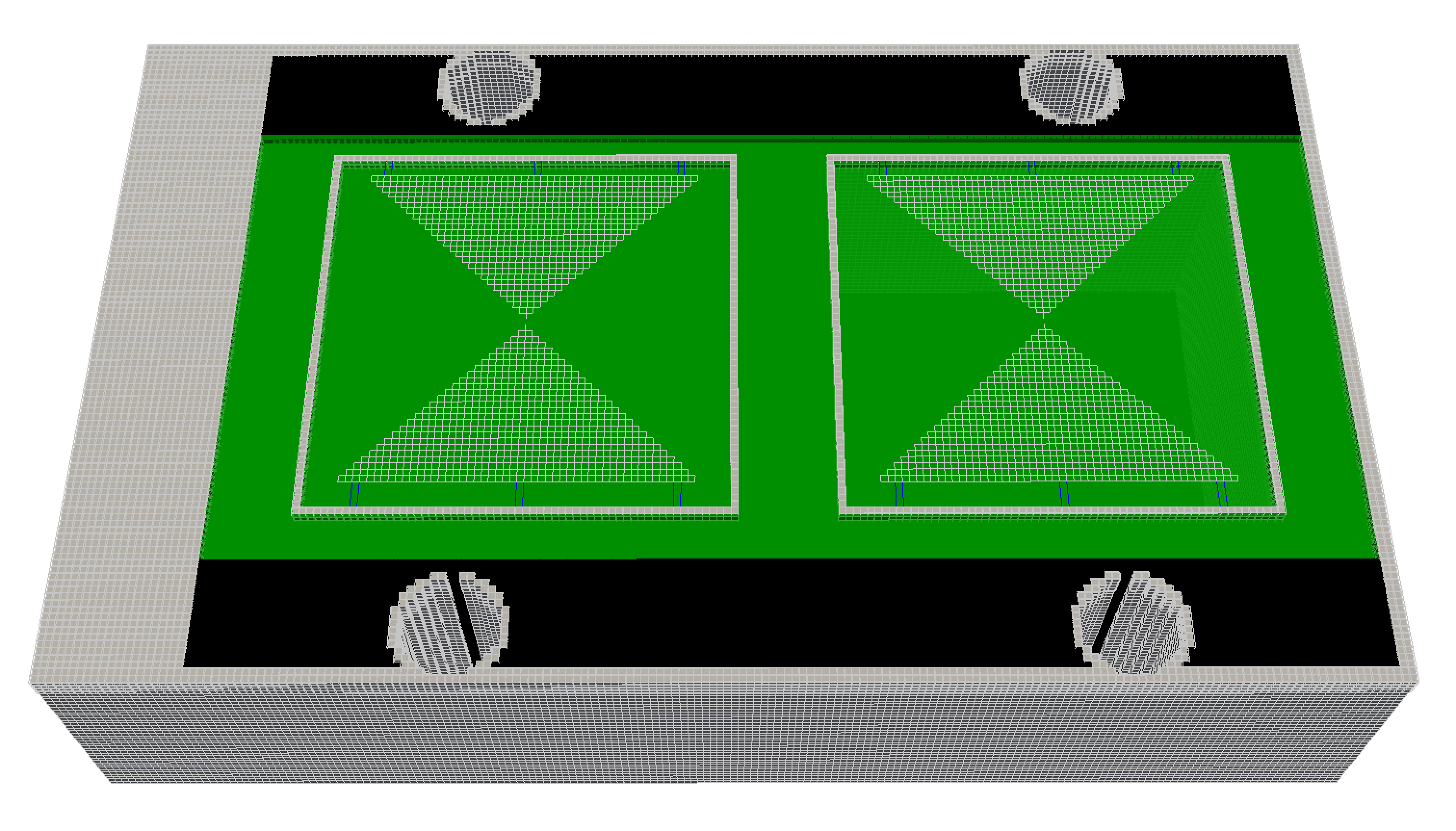
Fig. 58 FDTD geometry mesh showing an antenna model similar to a MALA 1.2GHz antenna (skid removed for illustrative purposes).