Frequency-Modulated Continuous-Wave GPR

Information

Receiver selections accept name:label and study:id as well as paths. An omitted background/incident receiver is matched by identity, not by the target’s numeric path. Explicit background selections are intentional per-file overrides. Missing/ambiguous identity is rejected. See Receiver numbering and cross-version processing for old/new output compatibility.

This toolbox synthesises frequency-modulated continuous-wave (FMCW) GPR outputs from one broadband gprMax simulation. It follows the short-pulse FDTD method of Eide et al. [EID2022FMCW], including background removal, source deconvolution, instrument correction, sweep apodisation, and conversion to fast time. It also provides ideal complex stretch-receiver I/Q samples for general linear-FMCW studies.

The method does not run a long chirp through FDTD. A static linear FDTD model has a channel response \(H(f)\) that can be measured efficiently with an impulse or another short broadband waveform. Every frequency in a linear chirp then samples this same channel. This avoids an FDTD time window comparable to a hardware sweep, which can be many orders of magnitude longer than the electromagnetic transient of interest.

Paper-equivalent processing

For an FDTD excitation \(w_{\mathrm{FDTD}}(t)\), subsurface reflectivity \(r(t)\), direct-wave coefficient \(d_d\), direct delay \(t_d\), and source artefact \(\gamma_w(t)\), Eide et al. write

\[y_{\mathrm{FDTD}}(t) = w_{\mathrm{FDTD}}(t) * \left[r(t) + d_d\delta(t-t_d)\right] + \gamma_w(t).\]

An empty or reference-model simulation supplies the direct wave and source artefact. After subtraction,

\[y_{\mathrm{target}}(t)-y_{\mathrm{background}}(t) = w_{\mathrm{FDTD}}(t)*r(t).\]

The toolbox first transforms the target and background records and divides each by its own exact stored source spectrum. It then subtracts the two normalised responses. This order is slightly more robust than subtracting raw records first because it remains correct if nominally identical runs have different sampled source amplitudes or time origins. With the engineering convention \(\Re\{X\exp(+j\omega t)\}\),

\[H(f) = \frac{Y(f)}{W(f)},\]

where source and receiver Yee-time offsets are read from the HDF5 output and included in the Fourier phase.

The processed FMCW spectrum is

\[Y_p(f) = A(f) I(f) H(f),\]

where \(A(f)\) is the sweep window and \(I(f)\) is an optional complex instrument transfer function. The fast-time response is its inverse discrete Fourier transform. This is the discrete form of (17) in [EID2022FMCW].

The supplied instrument response is deliberately user-defined. The toolbox does not claim to contain a RIMFAX calibration. RIMFAX is a gated FMCW radar covering 150–1200 MHz [HAM2020RIMFAX]; a measured or designed response can be supplied when that instrument is being represented.

Linear chirp and stretch receiver

For lower frequency \(f_0\), bandwidth \(B\), and sweep duration \(T\), the analytic up-chirp is

\[w(\tau) = \widetilde{i}(\tau) \exp\left\{j\left[2\pi f_0\tau +\pi\frac{B}{T}\tau^2\right]\right\}.\]

A reflector with delay \(t_i\) produces the deramped term

\[z_i(\tau) = a_i \exp\left(j2\pi\frac{B}{T}t_i\tau\right) \exp\left(-j\pi\frac{B}{T}t_i^2\right).\]

The first exponential has beat frequency \(f_b=(B/T)t_i\). The second is residual video phase (RVP). It is normally negligible for subsurface delays and long hardware sweeps, as assumed in [EID2022FMCW]. The toolbox can nevertheless include RVP on its discrete delay grid for experimental short, steep chirps. A later instrument-processing stage can compensate it by applying the opposite quadratic phase.

--deramped stores the ideal analytic stretch-receiver signal. Its I and Q datasets are real and imaginary parts under a convention giving a positive beat frequency for a delayed target during an up-chirp. The direct fast-time and explicit stretch-receiver routes are algebraically equivalent when RVP is neglected; this is checked automatically in the test suite.

Frequency and delay axes

For \(N\) sweep samples the toolbox uses the endpoint-exclusive grid

\[f_k = f_0 + \frac{B}{N}k, \qquad k=0,\ldots,N-1.\]

Consequently,

\[\Delta t_{\mathrm{fast}} = \frac{1}{B},\]

\[T_{\mathrm{unambiguous}} = \frac{N}{B}.\]

The delay resolution depends on bandwidth, not sweep duration. The sweep duration controls chirp slope and maps delay to beat frequency. A homogeneous two-way range axis can be requested with relative permittivity \(\epsilon_r\), using

\[R = \frac{c}{2\sqrt{\epsilon_r}}t.\]

For layered or dispersive media this range is only a display approximation; the stored delay axis is authoritative.

Preparing target and background models

An impulse is the most direct excitation, but any stored broadband source is valid over frequencies where its spectrum is sufficiently strong. The FDTD time window must capture the physical transient and its relevant late arrivals; it does not have to equal the FMCW sweep duration.

For a discrete plane wave, or another excitation without a scalar stored- source history, add --incident-reference and supply its empty/reference run with --background. The toolbox then calculates

\[H_{\mathrm{scattered}}(f) = \frac{Y_{\mathrm{total}}(f)-Y_{\mathrm{incident}}(f)} {Y_{\mathrm{incident}}(f)}.\]

The target and incident receiver coordinates and components must represent the same observation point. This is the route used by the retained analytical plane-wave validation.

The examples directory contains a small 2D layered target and its empty background:

• layered_fmcw_2D.in;

• layered_fmcw_background_2D.in.

Run both models and inspect the stored paths:

python -m gprMax gprMax/toolboxes/FMCW/examples/layered_fmcw_2D.in
python -m gprMax gprMax/toolboxes/FMCW/examples/layered_fmcw_background_2D.in
python -m gprMax.toolboxes.FMCW inspect layered_fmcw_2D.h5

Then synthesise a RIMFAX-band-like 100 ms up-chirp:

python -m gprMax.toolboxes.FMCW process layered_fmcw_2D.h5 \
    --background layered_fmcw_background_2D.h5 \
    --source /srcs/src1 --receiver /rxs/rx1 --component Ez \
    --f-start 150e6 --f-stop 1.2e9 --samples 1024 \
    --sweep-time 100e-3 --window blackman --tail-taper 0.05 --deramped \
    --output layered_fmcw_2D_fmcw.h5 \
    --plot layered_fmcw_2D_fmcw.png

Instrument and receiver responses

--instrument-response accepts a CSV frequency response with either

frequency_hz,real,imag

or

frequency_hz,magnitude,phase_deg

Complex interpolation is performed in magnitude and unwrapped phase. The file must cover the complete requested band.

--receiver-delay-response accepts delay_s plus gain, real,imag, or magnitude,phase_deg. It can represent range gating or an IF/ADC response after beat frequency has been mapped to delay. Keeping this separate from \(I(f)\) avoids confusing RF frequency-dependent antenna or electronics corrections with beat/delay-dependent receiver behaviour.

Output

The processed HDF5 file stores:

• chirp limits, slope, duration, direction, and endpoint convention;

• target and optional background source/receiver spectra;

• the source-normalised, background-subtracted channel_response;

• instrument response, sweep weights, processed spectrum, complex envelope, complex/real bandpass responses, and delay/range under fast_time; and

• optional complex signal, I/Q, instantaneous frequency, beat-frequency bins, and mapped delays under deramped_sweep.

Analytical multilayer validation

testing/validation/fmcw/validate_paper_multilayer.py is a canonical 2D validation inspired by the lossless multilayer processing sequence in Fig. 4 of [EID2022FMCW]. It is not an exact reproduction of the paper’s 3D bistatic antenna experiment. An empty gprMax model supplies the incident field; a fine-grid multilayer model supplies the total field; and their ratio is compared with the exact recursive normal-incidence reflection coefficient, including propagation phase and all internal reflections. The calculation uses the paper’s 150–1200 MHz band, 100 ms sweep duration, and Blackman taper.

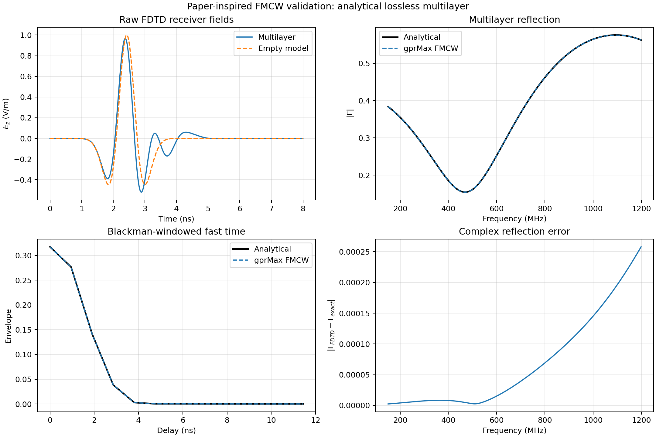
Fig. 90 Broadband gprMax fields, the source-normalised multilayer response, and the corrected fast-time result compared with the analytical multilayer solution.

For a 1 mm grid in double precision on CUDA, the complex relative error over the full band is \(2.46\times10^{-4}\), the magnitude RMSE is \(8.98\times10^{-5}\), and the Blackman-windowed fast-time complex error is \(1.38\times10^{-4}\). The small remaining difference grows smoothly with frequency and is attributable to FDTD spatial/time discretisation; the direct and explicit stretch-processing implementations agree to floating- point precision in the unit tests.

Scope and limitations

The method is exact for the sampled linear, time-invariant FDTD system over a valid source bandwidth and a sufficiently long transient record. It naturally includes linear material dispersion, antennas, PMLs, and scattering in the calculated channel.

One channel response does not by itself model target motion between chirps, Doppler evolution, oscillator phase noise, nonlinear receiver saturation, ADC quantisation, or time-varying media. Those effects can be applied to a sequence of channel responses or to the stored synthetic I/Q in a subsequent instrument model. Up- and down-chirps are supported, but triangular multi-ramp waveforms are assembled by processing their constituent sweeps.