Toolboxes is a sub-package where useful Python modules contributed by users are stored.

DebyeFit

Information

Author/Contact: Iraklis Giannakis (iraklis.giannakis@abdn.ac.uk), University of Aberdeen, UK and Sylwia Majchrowska (Sylwia.Majchrowska1993@gmail.com)

This module was created as part of the Google Summer of Code programme 2021 which gprMax participated.

License: Creative Commons Attribution-ShareAlike 4.0 International License

Attribution/cite: Giannakis, I., & Giannopoulos, A. (2014). A novel piecewise linear recursive convolution approach for dispersive media using the finite-difference time-domain method. IEEE Transactions on Antennas and Propagation, 62(5), 2669-2678. (http://dx.doi.org/10.1109/TAP.2014.2308549)

Electric permittivity is a complex function with both real and imaginary parts. In general, as a hard and fast rule, the real part dictates the velocity of the medium while the imaginary part is related to the electromagnetic losses. The generic form of dispersive media is

\[\epsilon(\omega) = \epsilon^{'}(\omega) - j\epsilon^{''}(\omega),\]

where \(\omega\) is the angular frequency, \(\epsilon^{'}\) and \(\epsilon^{''}\) are the real and imaginary parts of the permittivity respectively.

This package provides scripts and tools which can be used to fit a multi-Debye expansion to dielectric data, defined as

\[\epsilon(\omega) = \epsilon_{\infty} + \sum_{i=1}^{N}\frac{\Delta\epsilon_{i}}{1+j\omega t_{0,i}},\]

where \(\epsilon(\omega)\) is frequency dependent dielectric permittivity, \(\Delta\epsilon\) - difference between the real permittivity at zero and infinite frequency. \(\tau_{0}\) is relaxation time (seconds), \(\epsilon_{\infty}\) - real part of relative permittivity at infinite frequency, and \(N\) is number of the Debye poles.

To fit the data to a multi-Debye expansion, you can choose between Havriliak-Negami, Jonscher, or Complex Refractive Index Mixing (CRIM) models, as well as arbitrary dielectric data derived experimentally or calculated using a different function.

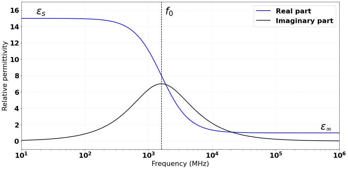
_images/epsilon.png — Fig. 63 Real and imaginary parts of frequency-dependent permittivity

Package contents

There are two main scripts:

Debye_Fit.py contains definitions of the relaxation function classes
optimization.py contains definitions of the three global optimization methods

Relaxation Class

This class is designed for modelling different relaxation functions, like Havriliak-Negami (HavriliakNegami), Jonscher (Jonscher), Complex Refractive Index Mixing (CRIM) models, and arbitrary dielectric data derived experimentally or calculated using some other function (Rawdata).

More about the Relaxation class structure can be found in the Relaxation documentation.

Havriliak-Negami Function

The Havriliak-Negami relaxation is an empirical modification of the Debye relaxation model in electromagnetism, which in addition to the Debye equation has two exponential parameters

\[\epsilon(\omega) = \epsilon_{\infty} + \frac{\Delta\epsilon}{\left(1+\left(j\omega t_{0}\right)^{a}\right)^{b}}\]

The HavriliakNegami class has the following structure:

HavriliakNegami(f_min, f_max,
                alpha, beta, e_inf, de, tau_0,
                sigma, mu, mu_sigma, material_name,
                number_of_debye_poles=-1, f_n=50,
                plot=False, save=False,
                optimizer=PSO_DLS,
                optimizer_options=None)

f_min is first bound of the frequency range used to approximate the given function (Hz),
f_max is second bound of the frequency range used to approximate the given function (Hz),
alpha satisfies \(0 < \alpha \leq 1\),
beta satisfies \(0 < \beta \leq 1\),
e_inf is a real part of relative permittivity at infinite frequency,
de is a difference between the real permittivity at zero and infinite frequency,
tau_0 is a relaxation time (seconds),
sigma is a conductivity (Siemens/metre),
mu is a relative permeability,
mu_sigma is a magnetic loss (Ohms/metre),
material_name is the material name,
number_of_debye_poles is the chosen number of Debye poles,
f_n is the chosen number of frequences,
plot is a switch to turn on the plotting,
save is a switch to turn on saving final material properties,
optimizer is a chosen optimizer to fit model to dielectric data,
optimizer_options is a dict for options of chosen optimizer.

Jonscher Function

Jonscher function is mainly used to describe the dielectric properties of concrete and soils. The frequency domain expression of Jonscher function is given by

\[\epsilon(\omega) = \epsilon_{\infty} + a_p\left(\frac{\omega}{\omega_p}\right)^{n_p-1} \left[1-j\cot\left(\frac{n_p\pi}{2}\right)\right]\]

The Jonscher class has the following structure:

Jonscher(f_min, f_max,
        e_inf, a_p, omega_p, n_p,
        sigma, mu, mu_sigma,
        material_name, number_of_debye_poles=-1,
        f_n=50, plot=False, save=False,
        optimizer=PSO_DLS,
        optimizer_options=None)

f_min is first bound of the frequency range used to approximate the given function (Hz),
f_max is second bound of the frequency range used to approximate the given function (Hz),
e_inf is a real part of relative permittivity at infinite frequency,
a_p is a Jonscher parameter. Real positive float number,
omega_p is a Jonscher parameter. Real positive float number,
n_p Jonscher parameter, 0 < n_p < 1.

Complex Refractive Index Mixing (CRIM) Function

CRIM is the most mainstream approach for estimating the bulk permittivity of heterogeneous materials and has been widely applied for GPR applications. The function takes form of

\[\epsilon(\omega)^{d} = \sum_{i=1}^{m}f_{i}\epsilon_{m,i}(\omega)^{d}\]

The CRIM class has the following structure:

Crim(f_min, f_max, a, volumetric_fractions,
    materials, sigma, mu, mu_sigma, material_name,
    number_of_debye_poles=-1, f_n=50,
    plot=False, save=False,
    optimizer=PSO_DLS,
    optimizer_options=None)

f_min is first bound of the frequency range used to approximate the given function (Hz),
f_max is second bound of the frequency range used to approximate the given function (Hz),
a is a shape factor,
volumetric_fractions is a volumetric fraction for each material,
materials are arrays of materials properties, for each material [e_inf, de, tau_0].

Rawdata Class

This package also has the ability to model dielectric properties obtained experimentally by fitting multi-Debye functions to data given from a file. The file must have at least two rows and exactly three numeric columns: frequency in Hz, real relative permittivity \(\epsilon'\), and the non-negative loss \(\epsilon''\) in the convention \(\epsilon = \epsilon' - j\epsilon''\). Do not supply the signed, negative imaginary component in column three. Values must be finite, frequencies positive and distinct, and \(\epsilon' \geq 1\). Rows are sorted by frequency before linear interpolation onto the logarithmic fitting grid. Duplicate frequencies must be combined by the user first. The default separator is a comma; delimiter selects another separator.

The Rawdata class has the following structure:

Rawdata(filename,
        sigma, mu, mu_sigma,
        material_name, number_of_debye_poles=-1,
        f_n=50, delimiter =',',
        plot=False, save=False,
        optimizer=PSO_DLS,
        optimizer_options=None)

filename is a path to text file which contains three columns,
delimiter is a separator for three data columns.

Important

sigma is an additional constant conductivity, written to the #material hash command. DebyeFit does not subtract it from the supplied loss data and does not include it in the fitted relaxation curve or its reported error. The exported material therefore has

\[\epsilon_{\mathrm{total}}(\omega) = \epsilon_{\mathrm{fit}}(\omega) - j\frac{\sigma}{\omega\epsilon_0}.\]

For measured data that already include all conduction loss, use sigma=0. Alternatively, subtract the known \(\sigma/(\omega\epsilon_0)\) from the positive loss column first, then pass that conductivity as sigma. The residual loss must remain non-negative. Rawdata warns when sigma is nonzero to prevent accidental double-counting. The analytical relaxation models use the same additive conductivity convention.

If a measurement table reports effective conductivity in S/m instead of dimensionless dielectric loss, first convert it using \(\epsilon''(f)=\sigma_{\mathrm{eff}}(f)/(2\pi f\epsilon_0)\). A loss-tangent column instead requires \(\epsilon''(f)=\epsilon'(f)\tan\delta(f)\). Neither column can be passed unchanged as Rawdata’s third column. When fitting the total converted loss, use sigma=0 as above.

Validation and interpreting a fit

Invalid model parameters raise ValueError rather than terminating Python. Frequency bounds must be finite, positive and distinct (reversed bounds are accepted). f_n must be an integer of at least two. Pole count is a positive integer or -1 for automatic selection. Relative permeability must be at least one; conductivity and magnetic loss must be finite and non-negative. Material names must also be valid, non-reserved gprMax identifiers without whitespace. Each run revalidates current parameter values, including edits made after construction.

run() returns (error_percent, hash_commands). The reported error is the sum of the two mean absolute normalised errors:

\[100\,\mathrm{mean}\!\left(\frac{|\epsilon'_{\mathrm{fit}}-\epsilon'|}{1+\epsilon'}\right) +100\,\mathrm{mean}\!\left(\frac{|\epsilon''_{\mathrm{fit}}-\epsilon''|}{1+|\epsilon''|}\right).\]

This is not a maximum-error bound or a pure relative percentage error. The plot shows signed normalised residuals, without the factor of 100. Automatic selection tries one through twenty poles and stops at a combined mean error of at most 5%; reaching twenty poles without meeting this target emits a warning. Check the curves and an independent, denser frequency grid before using a fit outside the sampled frequencies. Extrapolation beyond the fitted band is not validated.

The returned list contains a #material hash command and, when needed, a #add_dispersion_debye hash command. Exactly zero-strength poles are omitted; a lossless constant fit needs only #material. fitted_pole_count records the exported count, which can be smaller than the requested/trial number_of_debye_poles. Positive strengths are not thresholded away. Relaxation times in the exported command are in seconds, not their logarithms.

Saving is off by default. To choose the destination explicitly, use setup.save_result(hash_commands, fdir="existing_directory"). This appends to my_materials.txt; use unique material names when combining results. An explicit missing directory raises FileNotFoundError and does not fall back to another location. Omitting fdir retains the legacy search through ../materials, materials and user_libs/materials relative to the current working directory.

Class Optimizer

This class supports global optimization algorithms (particle swarm, dual annealing, evolutionary algorithms) for finding an optimal set of relaxation times that minimise the error between the actual and the approximated electric permittivity, and calculates optimised weights for the given relaxation times. Code written here is mainly based on external libraries, like scipy and pyswarm.

More about the Optimizer class structure can be found in the optimisation documentation.

PSO_DLS Class

Creation of hybrid Particle Swarm-Damped Least Squares optimisation object with predefined parameters. The code is a modified version of the pyswarm package which can be found at https://pythonhosted.org/pyswarm/.

DA_DLS Class

Creation of Dual Annealing-Damped Least Squares optimisation object with predefined parameters. The class is a modified version of the scipy.optimize package which can be found at: https://docs.scipy.org/doc/scipy/reference/generated/scipy.optimize.dual_annealing.html#scipy.optimize.dual_annealing.

DE_DLS Class

Creation of Differential Evolution-Damped Least Squares object with predefined parameters. The class is a modified version of the scipy.optimize package which can be found at: https://docs.scipy.org/doc/scipy/reference/generated/scipy.optimize.differential_evolution.html#scipy.optimize.differential_evolution.

DLS function

DLS is a legacy name. The implementation uses linear least squares for the imaginary-part weights, takes the magnitudes of those weights, and estimates a real offset constrained to \(\epsilon_\infty \geq 1\). It is neither a Levenberg–Marquardt solver nor non-negative least squares. Taking magnitudes is a heuristic, not an optimal positivity-constrained fit; closely spaced trial poles can give poor residuals. The global optimizers search over relaxation times using the unnormalised real-plus-imaginary mean absolute residual, while automatic pole selection uses the normalised metric above. Always inspect the accepted fit’s residuals.

All optimizer adapters honour named objective arguments independently of dictionary insertion order. maxiter controls the requested iteration budget. A fixed seed is reproducible without resetting NumPy’s global random state. For DE_DLS(workers=2), use a picklable objective and protect the calling script with if __name__ == "__main__": for multiprocessing. Use updating="deferred" in both serial and parallel runs when comparing their results with the same seed.

How to use the package

Examples

In the examples directory you will find Jupyter notebooks, scripts, and data that demonstrate different cases of how to use the main script Debye_Fit.py:

example_DebyeFitting.ipynb presents simple cases of using all available implemented relaxation functions.
example_BiologicalTissues.ipynb presents simple cases of using Cole-Cole function for biological tissues.
example_ColeCole.py presents simple cases of using Cole-Cole function in case of 3, 5 and automatically chosen number of Debye poles.
Test.txt contains raw data for testing the Rawdata class: frequency (Hz), real relative permittivity, and positive dielectric loss \(\epsilon''\).

From a source checkout, the independent validation cases can be reproduced with:

python -m testing.validation.validate_debye_fit --output-dir debyefit-validation

This writes plots and a JSON report, checks the exported spectra on a denser frequency grid, and exits with a nonzero status if any accuracy or passivity check fails. The report records the seed and iteration budget for each case.

The following code shows a basic example of how to use the Havriliak-Negami function:

# set Havrilak-Negami function with initial parameters
setup = HavriliakNegami(f_min=1e4, f_max=1e11,
                        alpha=0.3, beta=1,
                        e_inf=3.4, de=2.7, tau_0=.8e-10,
                        sigma=0.45e-3, mu=1, mu_sigma=0,
                        material_name="dry_sand", f_n=100,
                        plot=True, save=False,
                        number_of_debye_poles=3,
                        optimizer_options={'swarmsize':30,
                                           'maxiter':100,
                                           'omega':0.5,
                                           'phip':1.4,
                                           'phig':1.4,
                                           'minstep':1e-8,
                                           'minfun':1e-8,
                                           'seed': 111,
                                           'pflag': True})
# run optimization
setup.run()